EXTRAPOLATION WITH A SELF-ORGANISING

LOCALLY INTERPOLATING MAP

Controlling nonlinear Processes with ambiguous inverse Behaviour

Helge Hülsen, Sergej Fatikow

Division of Microrobotics and Control Engineering, University of Oldenburg

Uhlhornsweg 84, 26111 Oldenburg, Germany

Keywords: Associative Networks, Self-Organisation, Self-Supervised Learning, Extrapolation.

Abstract: Besides their typical classification task, Self-Organizing Maps (SOM) can be used to approximate input-

output relations. They provide an economic way of storing the essence of past data into input/output support

vector pairs. In this paper the SOLIM algorithm (Self-Organising Locally Interpolating Map) is reviewed

and an extrapolation method is introduced. This framework allows finding one inverse of a nonlinear many-

to-one mapping by exploiting the inherent neighbourhood criteria of the SOM part. Simulations show that

the performance of the mapping including the extrapolation is comparable to other algorithms.

1 INTRODUCTION

Several derivates of Self-Organizing Maps (SOM)

have been successfully applied to the control of

nonlinear, dynamic processes, which can also have

ambiguous inverse system behaviour (Barreto 2003).

A very important enhancement of the classical

SOM from Kohonen (overview in (Kohonen 2001))

has been the Local Linear Map (LLM) from Ritter et

al. (Ritter 1992) that has been further developed and

applied to various problems in robotics (Moshou

1997) and system dynamics modelling (Principe

1998)(Cho 2003). An LLM not only divides an input

space into subspaces as a standard SOM does but

assigns a local linear model to each subspace and

thus performs a mapping to an output space. By de-

scending on the error function of the local models

better estimates for these models are found. Re-

markable was the ability of the algorithm to learn a

meaningful mapping for processes with an ambigu-

ous inverse behaviour. This effect results from ap-

plying Kohonen's self-organising rule to update the

local model that has been responsible for the output

and all of its neighbours. The drawbacks of the LLM

are its discontinuities in the mapping at the transi-

tions between neighboured local models and the

strong dependency of the learning performance on

the Jacobians that define the linear models.

To solve the discontinuity problem Aupetit et al.

developed a continuous version of the LLM, the

Continuous Self-Organizing Map (CSOM) (Aupetit

1999)(Aupetit 2000), but still the mapping and the

learning was depending on the Jacobians and, in

addition, depending on interpolation parameters.

Walter followed another approach by avoiding a

discretisation of the input space and sharing the in-

fluence of each model on the output (Walter

1997)(Walter 2000). The influences are found with

help of an optimisation algorithm. On one hand this

leads to a continuous mapping, which can be opti-

mised with respect to different user-defined criteria

to resolve ambiguities. On the other hand this opti-

misation can be a relatively high computational load

for high network dimensions. Furthermore, under

certain conditions, there are problems with extrapo-

lation and the continuity of the mapping.

The Self-Organising Locally Interpolating Map

(SOLIM) from the author (Hülsen 2004a)(Hülsen

2004b) interpolates between different models with-

out any additional parameters. Learning is per-

formed in a self-supervised structure, which can be

interpreted as identification with exchanged input

and output. The main drawback of this algorithm is

the high computational effort for big networks,

which is in great part due to the extrapolation princi-

ple. In addition, extrapolation was only performed in

173

Hülsen H. and Fatikow S. (2005).

EXTRAPOLATION WITH A SELF-ORGANISING LOCALLY INTERPOLATING MAP - Controlling nonlinear Processes with ambiguous inverse

Behaviour.

In Proceedings of the Second International Conference on Informatics in Control, Automation and Robotics - Signal Processing, Systems Modeling and

Control, pages 173-178

DOI: 10.5220/0001177801730178

 SciTePress

a small area around the main mapping area. This

paper will introduce a new extrapolation algorithm

for the SOLIM.

The paper is organised as follows: In the next

section the fundaments of the SOLIM algorithm will

be explained. In section three the new extrapolation

principle will be presented in detail, followed by

simulations in section four. The paper ends with the

conclusion.

2 SOLIM: SELF-ORGANIZING

LOCALLY-INTERPOLATING

MAP

The SOLIM is a framework that shall perform two

tasks in a control context (

Figure 1):

1. Map from a desired state of a process

actuation parameters

to reach that state.

2. Use that pair of measured state

and actua-

tion parameters

to adapt the mapping.

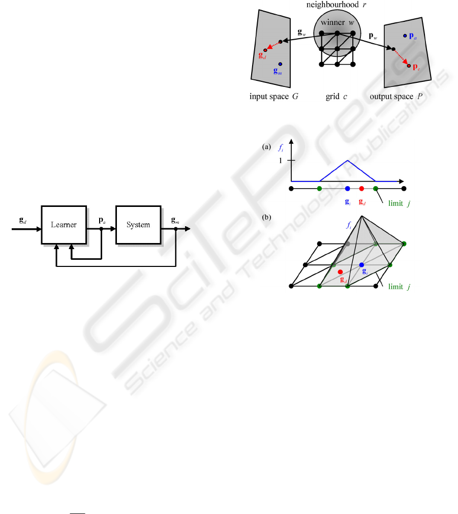
Figure 1: Self-supervised learning (Barreto 2004)

2.1 Mapping

As in a standard SOM (Hagan 1996), the base of

SOLIM is a grid

neurons with a certain

topology (Figure 2). Each neuron

is connected to

an input support vector

∈g and an output sup-

port vector

∈p . To perform the mapping

→

an influence weight

with respect to the input vec-

tor

is calculated for each neuron. The output

vector

is then the linear combination of all out-

put support vectors

f=⋅

∑

, (1.1)

where the weight

is scaled down to not exceed 1

if 1

otherwise

⎧

⎪

∑

⎨

⎪

⎩

∑

. (1.2).

The influence weights

are measures of how close

the input vector

is to the corresponding input

support vectors

. The influence weight is 1 for

and decreases to 0 at the limits of the influ-

ence range of neuron

(Figure 3).

Figure 2: Mapping and learning with self-organizing maps

(adopted from (Ritter 1992))

Figure 3: Influence

of neuron

for (a) a 1D grid in a

1D input space and (b) a 2D grid in a 2D input space

The limit

of an influence range is defined

solely by a selection of input support vectors

. For

the case of a 1D grid there are two limits for each

input support vector (

Figure 3(a)). When the grid is

placed in a 1D input space the limits are points, in a

2D input space the limits are lines and in a 3D input

space the limits are planes. Now considering a 2D

grid there are six limits for each input support vector

(

Figure 3(b)). When the grid is placed in a 2D input

space the limits are lines and in a 3D input space the

limits are planes again. In input spaces with higher

dimensions the limits will be hyperplanes.

A limit

can generally be defined by a position

vector

and a plane normal

, whose calculation

can be found in (Hülsen 2004b). The influence

weight

with respect to a limit

is calculated

ICINCO 2005 - SIGNAL PROCESSING, SYSTEMS MODELING AND CONTROL

174

with help of the relative distance

of the input

vector

from

in the direction to the limit plane

()

ij d i

ij ij i

⋅−

ngg

. (1.3)

A blending function

()

jij

bd= sets the influence to

0 for

d > , to 1 for

d < and defines a transition

for

d<<, i.e. the change of the influence from

one neuron to another.

The influences to the limits

are then combined to

the influence of the neuron

on the output vector

()

min

f= . (1.4)

Finally, it should be noted that the limits are de-

fined in a way that for a 1D grid two neurons are

responsible for the output vector, for a 2D grid three

neurons are responsible, for a 3D grid four neurons

are responsible, and so on (see also (Hülsen 2004b)).

2.2 Learning

Learning is performed in the input space

as well

as in the output space

with help of the Kohonen

learning rule (Kohonen 2001). Following the rule

not only the support vector of the "winner-neuron"

is updated but to a certain extent

()

also

the support vectors belonging to a neighbourhood

in the grid

(see Figure 2). In case of learning in

the input space the winner

is the neuron with the

highest influence with respect to the input vector

, which in turn serves as an attractor for

and

its neighbours

()

() ( 1) () ( 1)

ii g gdi

hwir

νν νν

−−

=+⋅ ⋅−gg gg. (1.5)

is a learning constant that, as the neighbourhood

radius

, is decreased with time. In case of learning

in the output space the winner

is the neuron with

the highest influence with respect to the measured

process output

. Since the process input

be-

longs to

, it can be used to find an estimate

for

by solving (1.1) for

aii

≠

⎛⎞

=−⋅

⎜⎟

⎝⎠

∑

pp p

. (1.6)

then serves as attractor for

and its

neighbours during the Kohonen update rule

()

() ( 1) () ( 1)

ii p pei

hwir

νν νν

−−

=+⋅ ⋅−pp pp . (1.7)

The Kohonen learning rule is topology conserv-

ing, which means that support vectors of neurons

that are neighbours in the grid

become neighbours

in the input space and output space. This property is

an inherent criterion to resolve ambiguities in the

inverse system behaviour

→ , since neighbours

in the input space map to neighbours in the output

space.

3 EXTRAPOLATION WITH

SOLIM

The main contribution of this paper is to show that

extrapolation is possible within the context of the

SOLIM-algorithm. Like the SOLIM-interpolation

the extrapolation algorithm only needs to know the

support vectors in the input and output space to per-

form a reasonably accurate extrapolation. The learn-

ing algorithm can be adapted to this enhanced map-

ping in a straight-forward manner.

3.1 Mapping

The mapping for regions outside the grid of input

support vectors is performed by adding an extrapola-

tion component

to each support vector

prior

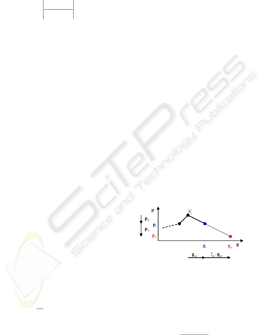
to interpolating between them (Figure 4)

()

iixi

f=⋅+

∑

ppp

. (1.8)

Figure 4: Extrapolation component

corresponds to

distance

l ⋅

of input vector from grid (1D grid)

The extrapolation component is computed as

ixin

l=⋅

, (1.9)

where

is a weight that defines the distance of the

input vector

from the input support vector

relation to

(Figure 4, Figure 5)

()

−

ggg

. (1.10)

EXTRAPOLATION WITH A SELF-ORGANISING LOCALLY INTERPOLATING MAP - Controlling nonlinear

Processes with ambiguous inverse Behaviour

175

is the mean difference vector between the input

support vector

and all input support vectors in its

limiting neighbourhood

()

iik

kN∈

=−

∑

ggg

. (1.11)

Analogously,

is the mean difference vector be-

tween the output support vector

and all output

support vectors in its limiting neighbourhood

()

iik

kN∈

=−

∑

ppp

. (1.12)

Figure 5: Calculation of

l ⋅

in a 2D grid

The main idea behind the interpolation as well as

the extrapolation mapping is that the relation be-

tween input vector and input support vector grid is

similar to the relation between output vector and

output support vector grid (Table 1). The weights

and

can therefore be applied in the input space in

the same way as in the output space. In addition,

since the calculation of the weights only depends on

the dimension of the grid

the mapping can be ap-

plied in both directions.

Table 1: Similarity of mapping in input and output space

input space output space

()

iixi

f≈⋅+

∑

ggg

()

iixi

f=⋅+

∑

ppp

ixin

l=⋅

ixin

l=⋅

()

iik

∈

=−

∑

ggg

()

iik

∈

=−

∑

ppp

3.2 Learning

The learning algorithm remains unchanged except

that the calculation of the estimation

for the sup-

port vector

that is most responsible for the sys-

tem output

(compare (1.6)) must take the ex-

trapolation components into account. Therefore (1.8)

must be solved for

, using (1.9) and (1.12)

()

aiixi

xw k

≠

∈

⎛⎞

−⋅+

⎜⎟

⎝⎠

⎜⎟

+⋅

⎜⎟

+⋅

⎜⎟

⎝⎠

∑

ppp

. (1.13)

It can be seen that when the extrapolation weight for

l = (1.13) becomes similar to (1.6), be-

cause no extrapolation is performed.

4 SIMULATIONS

The performance of the extrapolation algorithm can

be evaluated by mapping with support vectors that

represent a 2D Gaussian bell and by learning the

inverse of a well-known function.

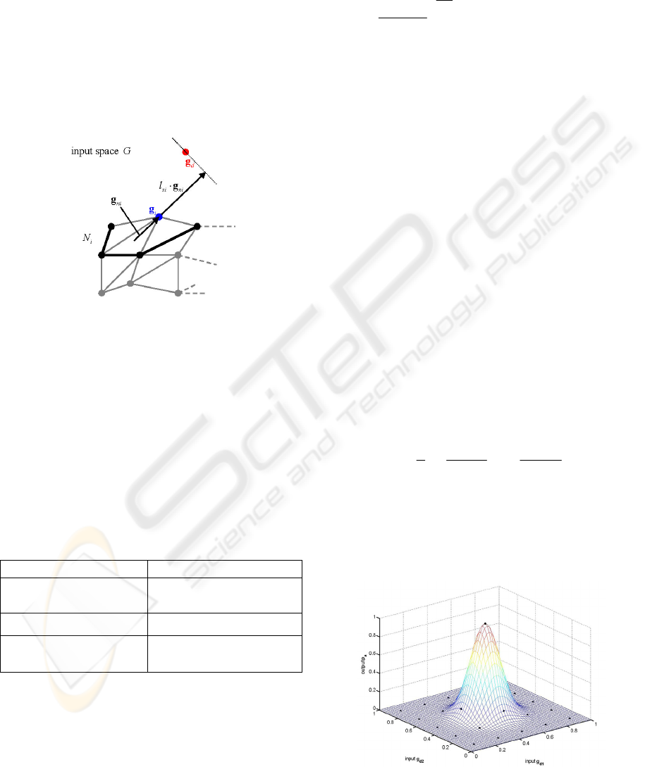
4.1 Mapping

For a performance measurement of the mapping 5x5

input support vectors

will be placed at the posi-

tions

{

}

,1 ,2

0.1,0.3,0.5,0.7,0.9

gg∈ . The corre-

sponding output support vectors

will be placed at

the corresponding positions of a 2D Gaussian bell

with

0.5

µ =

and

0.1

= (Figure 6)

,1 ,2

exp

gµ gµ

σσ

⎛⎞

−−

⎛⎞⎛⎞

⎜⎟

=−⋅ +

⎜⎟

⎜⎟⎜⎟

⎜⎟

⎝⎠⎝⎠

⎝⎠

p . (1.14)

For this support vector constellation the SOLIM

mapping in the range

[]

,1 ,2

0..

gg∈ is shown in

Figure 7. The RMS-error of 0.043 is comparable to

other algorithms as stated in Table 2.

Figure 6: 2D Gaussian bell in the range

[]

,1 ,2

,0..1

gg∈

ICINCO 2005 - SIGNAL PROCESSING, SYSTEMS MODELING AND CONTROL

176

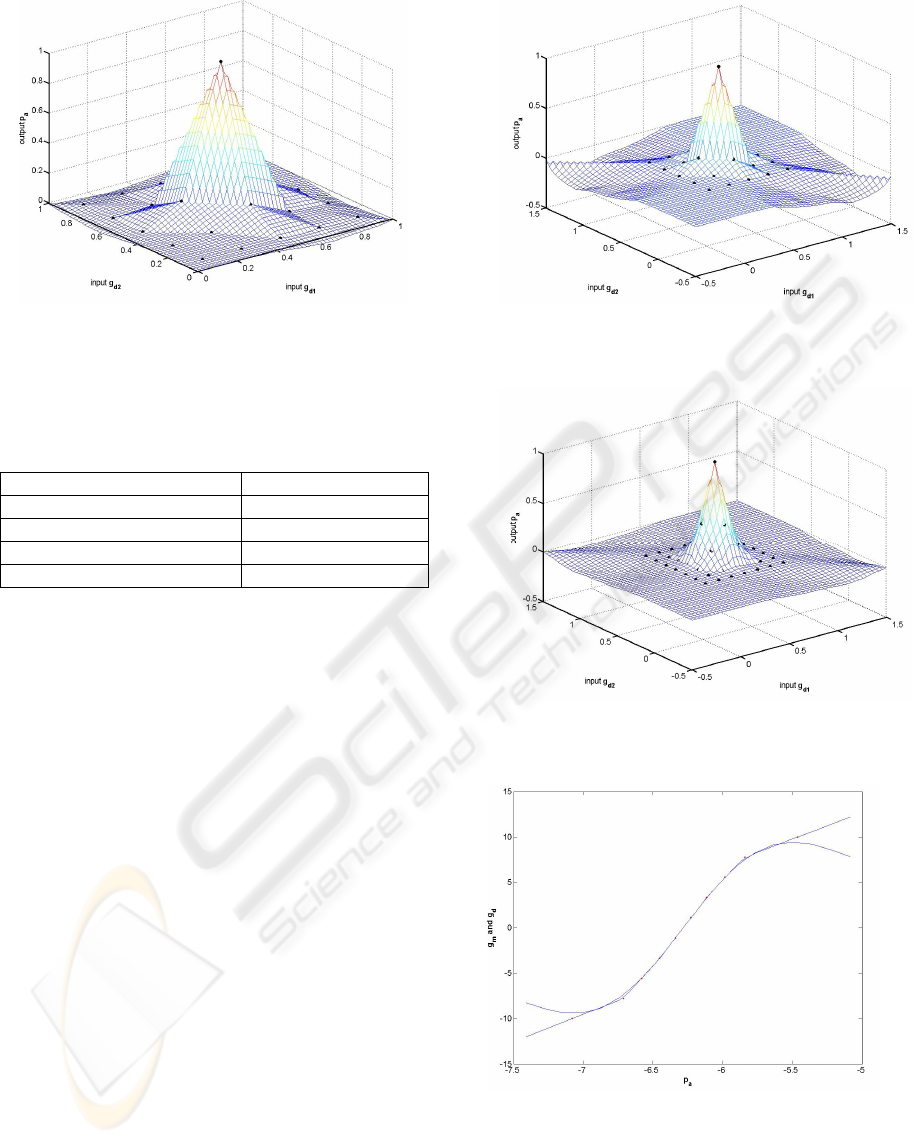
Figure 7: SOLIM-approximation (5x5 neurons) of 2D

Gaussian bell in the range

[]

,1 ,2

,0..1

gg∈

Table 2: RMS-error for approximation of 2D Gaussian

bell (

0.5

µ = ,

0.1

= ) with 25 support vectors in the

range

[]

,1 ,2

,0..1

gg∈ . Values from (Göppert 1997).

Algorithm RMS-error

local PSOM 0.049

RBF 0.041

CRI-SOM 0.016

SOLIM 0.043

To test the performance of the extrapolation

functions the same mapping is shown in Figure 8 for

a broader input range

[]

,1 ,2

0.5..1.

gg∈− . The

extrapolation is reasonable but the error is relatively

large (RMS-error = 0.063) because the falling slope

at the borders is continued although the Gaussian

bell approaches the zero-plane. This error can be

decreased significantly by using more neurons that

better represent the slopes, e.g. by placing 7x7 neu-

rons in the same area as shown in Figure 9 (RMS-

error = 0.025).

4.2 Learning

To validate the learning algorithm one inverse of the

function

()

= 10 sin(p) + 1/3 sin(3p

)

⋅⋅ (1.15)

shall be learned. In Figure 10 the result after 956

learning steps can be seen, where the RMS-error is

0.1% of the input vector range

[]

0..10

g ∈− . The

development of the error can be found in Figure 11.

It can be seen that the SOLIM algorithm with the

presented extrapolation can find one inverse to a

many-to-one, non-linear function.

Figure 8: SOLIM-approximation (5x5 neurons) of 2D

Gaussian bell in the range

[]

,1 ,2

, 0.5..1.5

gg∈−

Figure 9: SOLIM-approximation (7x7 neurons) of 2D

Gaussian bell in the range

[]

,1 ,2

, 0.5..1.5

gg∈−

Figure 10: Linear map with 10 neurons fits to

one inverse of (1.15) after 956 iteration steps.

RMS-error: 0.1% of

-range

EXTRAPOLATION WITH A SELF-ORGANISING LOCALLY INTERPOLATING MAP - Controlling nonlinear

Processes with ambiguous inverse Behaviour

177

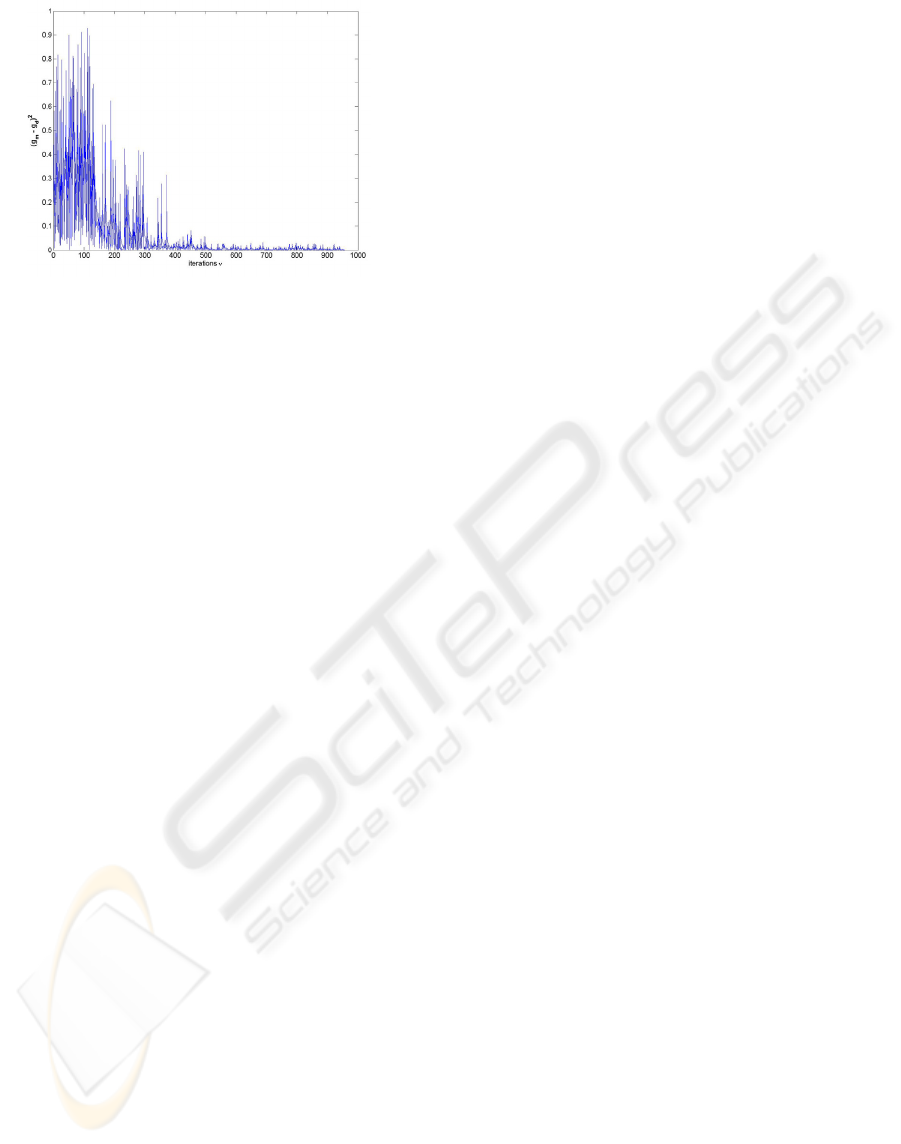
Figure 11: Development of RMS-error

5 CONCLUSION

It can be concluded that the presented algorithm has

the following properties:

• The extrapolation results from the interpolation

between the slopes at the borders, which is cal-

culated from the border support vectors and

their neighbours.

• The interpolation as well as the extrapolation

part only needs the input and output support

vectors to perform a mapping. No interpolation

factors and no local linear model matrices are

required. The price is that only 0-order continu-

ity is ensured, which mostly is sufficient.

• The mapping performance is comparable to

other algorithms (PSOM, RBF, ...).

• One mapping for ambiguous inverse system

behaviour can be found within a sufficient

number of iteration steps. Still a comparison to

other algorithms is missing since there is no

commonly accepted benchmark-system that can

be easily set up.

The following problems have not been solved yet:

• The topology is still fixed and must be known a-

priori. There exist algorithms that dynamically

build topologies and neighbourhood relation-

ships, depending on the input data "structure".

• There are still learning parameters that must be

tuned before each experiment and that partially

vary depending on time. For online training

these parameters must be varied automatically.

• The presented algorithm shall be tested in a real

application. One good demonstration is to learn

non-linear, time-variant and many-to-one mo-

tion characteristics of microrobots (Hülsen

2004a).

REFERENCES

Aupetit, M., Couturier, P., and Massotte, P. (1999). A

continuous self-organizing map using spline technique

for function approximation. In

Proc. Artificial Intelli-

gence and Control Systems (AICS'99)

, Cork, Ireland.

Aupetit, M., Couturier, P., and Massotte, P. (2000). Func-

tion approximation with continuous self-organizing

maps using neighboring influence interpolation. In

Proc. Neural Computation (NC'2000), Berlin, Ger-

many.

de A. Barreto, G., Araújo, A. F. R., and Ritter, H. J.

(2003). Self-organizing feature maps for modeling and

control of robotic manipulators.

Journal of Intelligent

and Robotic Systems

, 36(4):407-450.

de A. Barreto, G. and Araújo, A. F. R. (2004). Identifica-

tion and control of dynamical systems using the self-

organizing map.

IEEE Transactions on Neural Net-

works

, 15(5):1244-1259.

Cho, J., Principe, J. C., and Motter, M. A. (2003). A local

linear modeling paradigm with a modified counter-

propagation network. In

Proc. Int. Joint Conf. on Neu-

ral Networks

, pages 34-38, Portland, OR, U.S.A.

Hagan, M. T., Demuth, H. B., and Beale, M. (1996). Neu-

ral Network Design

. PWS Publishing Co., Boston,

MA, U.S.A.

Hülsen, H., Trüper, T., and Fatikow, S. (2004a). Control

system for the automatic handling of biological cells

with mobile microrobots. In

Proc. American Control

Conference (ACC'04)

, pages 3986-3991, Boston, MA,

U.S.A.

Hülsen, H. (2004b). Design of a fuzzy-logic-based bidirec-

tional mapping for kohonen networks. In

Proc. Int.

Symposium on Intelligent Control (ISIC'04)

, pages

425-430, Taipei, Taiwan.

Kohonen, T. (2001).

Self-Organizing Maps. Springer,

Berlin, Germany, 3. edition.

Moshou, D. and Ramon, H. (1997). Extended self-

organizing maps with local linear mappings for func-

tion approximation and system identification. In

Proc.

Workshop on Self-Organizing Maps (WSOM'97)

pages 181-186, Helsinki, Finland.

Principe, J. C., Wang, L., and Motter, M. A. (1998). Local

dynamic modelling with self-organizing maps and ap-

plications to nonlinear system identification and con-

trol.

Proceedings of the IEEE, 86(11):2240-2258.

Ritter, H., Martinetz, T., and Schulten, K. (1992).

Neural

Computation and Self-Organizing Maps: An Introduc-

tion

. Addison-Wesley, Reading, M.A., U.S.A.

Walter, J., Nölker, C., and Ritter, H. (2000). The PSOM

algorithm and applications. In

Proc. of Int. Symp. on

Neual Computation (NC'2000)

, pages 758-764, Berlin,

Germany.

Walter, J. (1997).

Rapid Learning in Robotics. Cuvillier

Verlag, Göttingen. http://www.techfak.uni-

bielefeld.de/ walter/.

ICINCO 2005 - SIGNAL PROCESSING, SYSTEMS MODELING AND CONTROL

178