
ROBUST CONTROL OF INDUCTION MOTOR USING FAST
OUTPUT SAMPLING TECHNIQUE
Alemayehu G/E Abera, B. Bandyopadhyay, S. Janardhanan
Systems and Control Engineering
IIT Bombay, Mumbai, INDIA
Vivek Agrawal
Dept. of Electrical Engineering
IIT Bombay, Mumbai, INDIA
Keywords:
Induction motor , fast output sampling, integral action, robust control.
Abstract:
In this paper a design method based on robust fast output sampling technique is presented for the speed control
of induction motor. The nonlinear model of induction motor model is linearized around various operating
points to obtain the linear models. The input of the induction motor is the stator voltages and only the speed is
considered as the output of the systems. A single controller is designed for these linear models. The nonlinear
model of the induction motor is simulated with the proposed controller at these operating points. This method
does not require the state of the system for feedback and is easily implementable.
1 INTRODUCTION
The induction motor is being used in many industrial
applications due to its reliability, ruggedness, and low
cost. Its mechanical reliability is due to the fact that
there is no mechanical commutation(i.e. there are no
brushes nor commutator to wear out as in a DC mo-
tor). Further more it can also be used in volatile envi-
ronments since no sparks are produced as is the case
with the commutator of a DC motor. For these and
other reasons induction motor is widely used in many
electric drive applications. However, the induction
motor presents a challenging control problem. This
is due to the fact that this dynamical system is nonlin-
ear, two of the state variables (rotor fluxes/currents)
are not usually measurable, and due to heating the
rotor resistance varies considerably with a signifi-
cant impact on the system dynamics. High perfor-
mance drives for various applications using induc-
tion motors with vector control have become the pre-
ferred form of motive power in a number of applica-
tions. Vector control transforms the induction motor
into a system that has the characteristics of a sepa-
rately excited DC motor. Success of vector control
techniques depend on the knowledge of instantaneous
magnitude and position of rotating magnetic field (or
flux) in the machine. Direct measurement of mag-
netic field using search coils, hall effect sensors re-
quire implantation of sensors in the air gap of the ma-
chine and hence result in increased complexity. More-
over, they are prone to errors caused by factors like
temperature variation and noise (Janson and Lorenz,
1992),(Verghese and Sanders).
In order to circumvent direct measurement of the
magnetic flux, a number of flux estimation methods
have been proposed in the last few years (Janson and
Lorenz, 1992),(Sangwongwanich et al.,). All these
methods utilize terminal measurements of voltage and
current along with (or without) rotor speed to arrive
at an accurate estimate of the magnitude and posi-
tion of the flux in the machine. These methods have
been broadly classified as open loop observers and
closed loop observers to have superior performance
characteristics with respect to robustness and accu-
racy(Janson and Lorenz, 1992). Almost all of the lit-
erature uses more than one of the system states for the
design of the controller.
In this paper a design of robust fast output sampling
controller for induction motor control by measuring
only the speed is proposed. This is done by sampling
the speed signal at a faster rate than the input signal. It
will be shown that using this technique a robous con-
trrol for the multimodel representation of nonlinear
model of the induction motor can be obtained. The
outline of the paper is as follows. Section 2 presents
dynamic model of an induction motor. Section 3 deals
with a brief introduction of fast output sampling con-
trol technique where as the controller design is pre-
sented in Section 4. Section 5 presents simulation re-
sults and discussions followed by the concluding re-
marks.
25
G/E Abera A., Bandyopadhyay B., Janardhanan S. and Agrawal V. (2005).
ROBUST CONTROL OF INDUCTION MOTOR USING FAST OUTPUT SAMPLING TECHNIQUE.
In Proceedings of the Second International Conference on Informatics in Control, Automation and Robotics - Robotics and Automation, pages 25-30
DOI: 10.5220/0001175600250030
Copyright
c
SciTePress

2 DYNAMIC MODEL OF AN
INDUCTION MOTOR
Under the commonly used assumptions, the behavior
of the three phase, four pole, induction motor in the
orthogonal field reference frame can be described by
a set of non-linear equations as given below (Kraus,
et al, 2002) ,(Mohan, 2000), (Mohan, 2001)
d
dt
i
ds
= σR
s
i
ds
+ ω
s
i
q s
+ βL
m
ω
r
i
q s
(1)
+βR
r
i
dr
+ βL
r
ω
r
i
q r
+ σV
ds
d
dt
i
q s
= −ω
s
i
ds
− βL
m
ω
r
i
ds
− σR
s
i
q s
−σL
m
ω
r
i
dr
+ βR
r
i
q r
+ σV
q s
d
dt
i
dr
= βR
s
i
ds
− γL
m
ω
r
i
q s
− γR
r
i
dr
+ω
s
i
q r
− σL
s
ω
r
i
q r
− βV
ds
d
dt
i
q r
= βL
s
ω
r
i
ds
+ βR
s
i
q s
− ω
s
i
dr
+σL
s
ω
r
i
dr
− γR
r
i
q r
− βV
q s
d
dt
ω
r
=
p
2J
eq
(T
e
− T
L
)
T
e
=
3
2
P
2
L
m
(i
q s
i
dr
− i
ds
i
q r
) .
where i
ds
, i
q s
are stator currents, i
dr
, i
q r
are rotor cur-
rents, V
ds
, V qs are stator voltages, ω
r
is rotor angle
velocity, ω
s
is synchronous speed, T
e
, T
L
are electro-
magnetic and load torques, J
eq
is inertia of the rotor,
p is number of poles, α, β, σ and γ are all positive
constants defined as:
α = L
s
L
r
− L
2
m
,
β = L
m
/α,
σ = L
r
/α,
γ = L
s
/α
where L
s
and L
r
are stator and rotor inductances, R
s
and R
r
are stator and rotor resistances and L
M
is the
mutual inductance. The output is the rotor speed.
3 ON FAST OUTPUT SAMPLING
FEEDBACK
3.1 Review on Fast Output
Sampling Feedback
The problem of simultaneous stabilization has re-
ceived considerable attention in the literature. Given
a family of plants in state space representation
(Φ
i
, Γ
i
) , i = 1, · · · , M, find a linear state feed-
back gain F such that (Φ
i
+ Γ
i
F ) is stable for i =
1, · · · , M , or determine that no such F exists. But
the method is of use only in the case where whole
state information is available.
One way of approaching this problem with incom-
plete state information is to use observer based control
laws, i.e. dynamic compensators. The problem here
is that the state feedback and state estimation cannot
be separated in face of the uncertainty represented by
a family of systems. Assuming that a simultaneously
stabilizing F has been found, it is possible to search
for a simultaneously stabilizing full order observer
gain, but this search is dependent on the F previously
obtained. If no stabilizing observer for this state feed-
back exists, nothing can be said because there may ex-
ist stabilizing observers for different feedback gains.
With the Fast output sampling approach proposed
by (Werner and Furuta, 1995) it is generically possi-
ble to simultaneously realize a given state feedback
gain for a family of linear, observable models. For
fast output sampling gain L realize the effect of state
feedback gain F , find the L such that (Φ
i
+ Γ
i
LC)
is stable for i = 1, · · · , M, If there exist a set of
F ’s, there should exist a common L for given fam-
ily of plants. One of the problems with this approach
is that large feedback gains tend to render the system
very noise -sensitive. To overcome this problem the
design problem can be posed as a multi-objective op-
timization problem in an LMI formulation proposed
by (Werner, 1998).
Consider a plant described by a linear model
.
x
= Ax + Bu, (2)
y = Cx, (3)
with (A, B) controllable and (C, A) observable.
Assume the plant is to be controlled by a digital con-
troller, with sampling time τ and zero order hold, and
that a sampled data state feedback design has been
carried out to find a state feedback gain F such that
the closed loop system
x (kτ + τ ) = (Φ
τ
+ Γ
τ
F )x (kτ ) , (4)
has desired properties. Hence Φ
τ
= e
Aτ
and
Γ
τ
=
R
τ
0
e
As
dsB. Instead of using a state observer,
the following sampled data control can be used to re-
alize the effect of the state feedback gain F by output
feedback. Let ∆ = τ /N, and consider
u(t) = [L
0
· · · , L
N−1
]
y (kτ − τ )
.
.
.
y (kτ − ∆)
= Ly
k
, (5)
for kτ ≤ t < (k + 1)τ , where the matrix blocks
L
j
represent output feedback gains, and the notation
ICINCO 2005 - ROBOTICS AND AUTOMATION
26

L, y
k
has been introduced for convenience. Note that
1/τ is the rate at which the loop is closed, whereas
output samples are taken at the N -times faster rate
1/∆.
To show how a fast output sampling controller (5
) can be designed to realize the given sampled-data
state feedback gain, we construct a fictitious, lifted
system for which (5 ) can be interpreted as static out-
put feedback. Let ( Φ, Γ, C ) denote the system (2) at
the rate 1/∆. Consider the discrete-time system hav-
ing at time t = kτ the input u
k
= u(kτ), state x
k
=
x(kτ) and output y
k
as
x
k+1
= Φ
τ
x
k
+ Γ
τ
u
k
, (6)
y
k+1
= C
0
x
k
+ D
0
u
k
, (7)
where
C
0
=
C
CΦ
.
.
.
CΦ
N−1
, D
0
=
0
CΓ
.
.
.
C
P
N−2
j=0
Φ
j
Γ
.
Assume that the state feedback gain F has been de-
signed that (Φ
τ
+ Γ
τ
F ) has no eigenvalues at the ori-
gin. Then, assuming that in intervals kτ ≤ t < kτ +τ
u(t) = F x(kτ), (8)
one can define the fictitious measurement matrix
C(F, N) = (C
0
+ D
0
F )(Φ
τ
+ Γ
τ
F )
−1
, (9)
which satisfies the fictitious measurement equation
y
k
= Cx
k
. For L to realize the effect of F , it must
satisfy
LC = F. (10)
Let ν denote the observability index of (Φ, Γ). It
can be shown that for N ≥ ν, generically C has full
column rank, so that any state feedback gain can be
realized by a fast output sampling gain L.
If the initial state is unknown, there will be an error
∆u
k
= u
k
- F x
k
in constructing the control signal
under state feedback. One can verify that the closed
loop dynamics are governed by
X
k+1
∆u
k+1
=
Φ
τ
+ Γ
τ
F Γ
τ
0 Ψ(L)
x
k
∆u
k
.
(11)
where Ψ(L) = LD
0
− F Γ
τ
.
Thus, one can say that the eigenvalues of the closed
loop system under a fast output sampling control law
(5) are those of Φ
τ
+ Γ
τ
F together with those of
LD
0
− F Γ
τ
.
One feature of fast output sampling control that
makes it attractive for robust controller design, is the
fact that a result similar to the above can be shown to
hold when the same state feedback is applied simul-
taneously to a family of models representing different
operating conditions of the plant.
3.2 Integral Action
The fast output controller (5), can be used to realize
the effect of state feedback. If step disturbances are
to be rejected with zero steady state error, then the
controller must integrate the tracking error. A pure
state feedback control law does not include integral
action, but can be made to do so by introducing a
new state ζ that integrates the error (Werner, 1996).
This can be realize in discrete time using:
ζ
k+1
= ζ
k
+ r
k
− y
k
where r
k
stands for the sampled reference input. A
discrete time state space representation for the aug-
mented system is
¯x(k + 1) =
¯
Φ¯x(k) +
¯
Γu(k) +
¯
Γ
r
r(k), (12)
where ¯x(k) = [x(k)
T
ζ
k
]
T
and
¯
Φ =
Φ
τ
0
−C I
,
¯
Γ =
Γ
τ
0
,
¯
Γ
r
=
0
I
.
State feedback gain F and the integrator gain F
I
can
be collected from a new state feedback gain
¯
F = [F
F
I
] to yield the control law
u(k) =
¯
F x(k) = F x(k) + F
I
ζ
k
= Ly
k
+ F
I
ζ
k
(13)
with a resulting closed loop matrix:
¯
Φ
τ
+
¯
Γ
τ
¯
F =
Φ
τ
+ Γ
τ
F Γ
τ
F
I
−C I
,
3.3 Multimodel Synthesis
For multimodel representation of a plant, it is nec-
essary to design controller which will robustly stabi-
lize the multimodel system. Multimodel representa-
tion of plants can arise in several ways. When a non-
linear system has to be stabilized at different operat-
ing points, linear models are sought to be obtained
at those operating points. Even for parametric un-
certain linear systems, different linear models can be
obtained for extreme points of the parameters or for
ROBUST CONTROL OF INDUCTION MOTOR USING FAST OUTPUT SAMPLING TECHNIQUE
27

family of different models. The models are used for
stabilization of different machine models
Now consider a family of plant S = {A
i,
B
i,
C
i
},
defined by
˙x = A
i
x + B
i
u, (14)
y = C
i
x, i = 1, · · · , M. (15)
By sampling at the rate of 1/△, we get a family of
discrete-time systems {Φ
i
, Γ
i
, C
i
}.
Consider the family of discrete-time systems given
by Eqns.(14) and (15) having at time t= kτ the input
u
k
= u(kτ), state x
k
= x(kτ) and output y
k
as
x
k+1
= Φ
τ i
x
k
+ Γ
τ i
u
k
, (16)
y
k+1
= C
0i
x
k
+ D
0i
u
k
, (17)
Assume that (Φ
τ i
, Γ
i
) are controllable. Then we
can find a robust state feedback gains F such that
(Φ
τ i
+ Γ
i
F ) has no eigenvalues at the origin.
Then, assuming that in intervals kτ ≤ t < kτ + τ
u(t) = F x(kτ), (18)
one can define the fictitious measurement matrix
C
i
(F, N) = (C
0i
+ D
0i
F )(Φ
τ i
+ Γ
τ i
F )
−1
, (19)
which satisfies the fictitious measurement equation
y
k
= C
i
x
k
. For robust fast output sampling gain L to
realize the effect of F , it may satisfy
LC
i
= F, i = 1, · · · , M. (20)
The Eqn.(20) can be written as
L
∽
C
=
∽
F
, (21)
where
∽
C
= [
C
1
C
2
· · · C
M
] ,
∽
F
= [
F F · · · F
] .
The robust state feedback gain F can be obtained
from the augmented matrix (12) by considering a fam-
ily of plants
¯
S =
¯
Φ
i
,
¯
Γ
i
,
¯
Γ
ri
, defined by.
¯x(k + 1) =
¯
Φ
i
¯x(k) +
¯
Γ
i
u(k) +
¯
Γ
ri
r(k), (22)
3.4 An LMI Formulation of the
Design Problem
When this idea is realized in practice i.e. fast out-
put sampling gain L have been obtained by realizing
the state feedback gain F , two problems are required
to be addressed. The first one is apparent from(11).
With this type of controller, the unknown states are
estimated implicitly, using the measured output sam-
ples and assuming that initial control is generated by
state feedback. If initial state causes an estimation
error, then decay of this error will be determined by
the eigenvalues of the matrix (LD
0i
− F Γ
τ i
) which
depends on L and whose dimension equals the num-
ber of control input. For stability these eigenvalues
have to be inside the unit disc, and for fast decay they
should be as close to the origin as possible. This prob-
lem must be taken into account while designing L.
The second problem is that the gain matrix L may
have elements with large magnitude. Because these
values are only weights in linear combination of out-
put samples, large magnitudes do not necessarily im-
ply large control signal, and in theory and noise free
simulation they pose no problem. But in practice they
amplify measurement noise, and it is desirable to keep
these values low. This objective can be expressed by
an upper bound ρ on the norm of the gain matrix L.
When trying to deal with these problem, it is bet-
ter not to insist on an exact solution to the design(20):
one can allow a small deviation and use an approx-
imation LC
i
≈F, which hardly affects the desired
closed-loop dynamics, but may have considerable ef-
fect on the two problems described above. Instead of
looking for an exact solution to the equalities, the fol-
lowing inequalities are solved
kLk < ρ
1
,
kLD
0i
− F Γ
τ i
k < ρ
2i
, i = 1, · · · , M,
kLC
i
−F k < ρ
3i.
(23)
Here three objectives have been expressed by upper
bounds on matrix norms, and each should be as small
as possible. The ρ
1
small means low noise sensitivity,
ρ
2
small means fast decay of estimation error, most
important - ρ
3
-small means that fast output sampling
controller with gain L is a good approximation of the
originally designed state feedback controller. If ρ
3
=
0 then L is exact solution.
Using the Schur complement, it is straight forward
to bring these conditions in the form of LMI (Linear
Matrix Inequalities) proposed by (Werner, 1996)
−ρ
2
1
I L
L
T
−I
< 0,
−ρ
2
2i
I (LD
0i
− F Γ
τ i
)
(LD
0i
− F Γ
τ i
)
T
−I
< 0,
−ρ
2
3i
I (LC
i
−F)
(LC
i
−F)
T
−I
< 0. (24)
In this form, the function mincx() of the LMI con-
trol toolbox for MATLAB can be used immediately
ICINCO 2005 - ROBOTICS AND AUTOMATION
28

to minimize a linear combination of ρ
1
, ρ
2
, ρ
3
. The
following approach turned out to be useful. If the
actual measurement noise is known, the magnitude
of L is fixed accordingly. Likewise eigenvalues of
(LD
0i
− F Γ
τ i
) less than 0.05 cause no problem. So
we can fix ρ
1
, ρ
2
and only ρ
3
is minimized subject to
these constraints.
In this form the LMI Tool Box of MATLAB can
be used for synthesis as suggested by (Gehenet, et al.,
1995).
The fast output sampling feedback controller ob-
tained by the above method requires only constant
gains and hence is easier to implement. The example
of multi machine system dynamics is used to demon-
strate the method.
4 CONTROLLER DESIGN
The design procedure assumes a linear model. The
linearization was carried out about an operating point
of the non-linear induction motor model (1), with the
data provided in the appendix for three induction ma-
chine models.
Since the nonlinear system is to track a constant
reference speed, the linear system composed of the
error states, obtained at this nominal speed would be
equivalently required to track a reference of zero. The
continuous linear models are discretized and the dis-
crete models are represented by the following equa-
tion
∆x(k + 1) = Φ
τ i
∆x(k) + Γ
τ i
∆u(k), (25)
∆y(k) = C
i
∆x(k), i = 1, 2, 3 (26)
where
∆x(k) = [
∆i
ds
∆i
q s
∆ω
r
∆i
ds
∆i
q s
]
T
∆u(k) = [
∆V
ds
∆V
q s
]
T
with the speed of the induction machines being the
output. The appropriate control action can now be
computed using Eqn. (13).
However, for tracking of a reference speed, the in-
tegral action F
I
ζ
k
would require the error in the speed
of the system. This is realized by comparing the ac-
tual speed with the reference speed.
and
∆u(k) = F
I
ζ (k) + L∆y
k
(27)
From the incremental control ∆u(k), actual control
u(k) is obtained.
u(k) = u
0
+ ∆u
k
5 SIMULATION RESULTS AND
DISCUSSIONS
The system (1) is linearized about three operating
points using MATLABr to get a linear system of
form (14), Discretization of (A
i
, B
i
, C
i
) at an inter-
val of τ = 0.04 sec . and adding an integrator leads
to the augmented system (22) for which a common
state feedback gain must be found. This problem
can be solved by convex programming methods,for
which software tools are available in the LMI toolbox
for Matlab(Gehenet, et al., 1995). This yields a state
feedback gain:
¯
F = [F F
I
] =
=
−0.1227 25.8298 37.6501 · · ·
−2.9221 72.7314 42.1827 · · ·
· · · 27.5299 38.8149 7.4603
· · · 74.0091 42.0990 1.2915
Using (21), the fast output sampling gain is calcu-
lated as
L =
−6.128 22.643 −29.69 5.858
−2.075 10.899 −23.982 12.78
..
..
22.365 −9.549 −21.152 6.531
19.153 −15.18 −19.264 13.476
..
..
18.73 −6.51 −18.668 11.02
21.415 −10.677 −23.443 10.585
..
21.403 −31.972 12.87
22.504 −33.03 15.132
Now, using Eqn. (27), ∆u(k) is obtained and u(k) for
the nonlinear model which is u
0
+ ∆u(k) is also ob-
tained. This is used in the simulation of the nonlinear
model with 10% change in load.
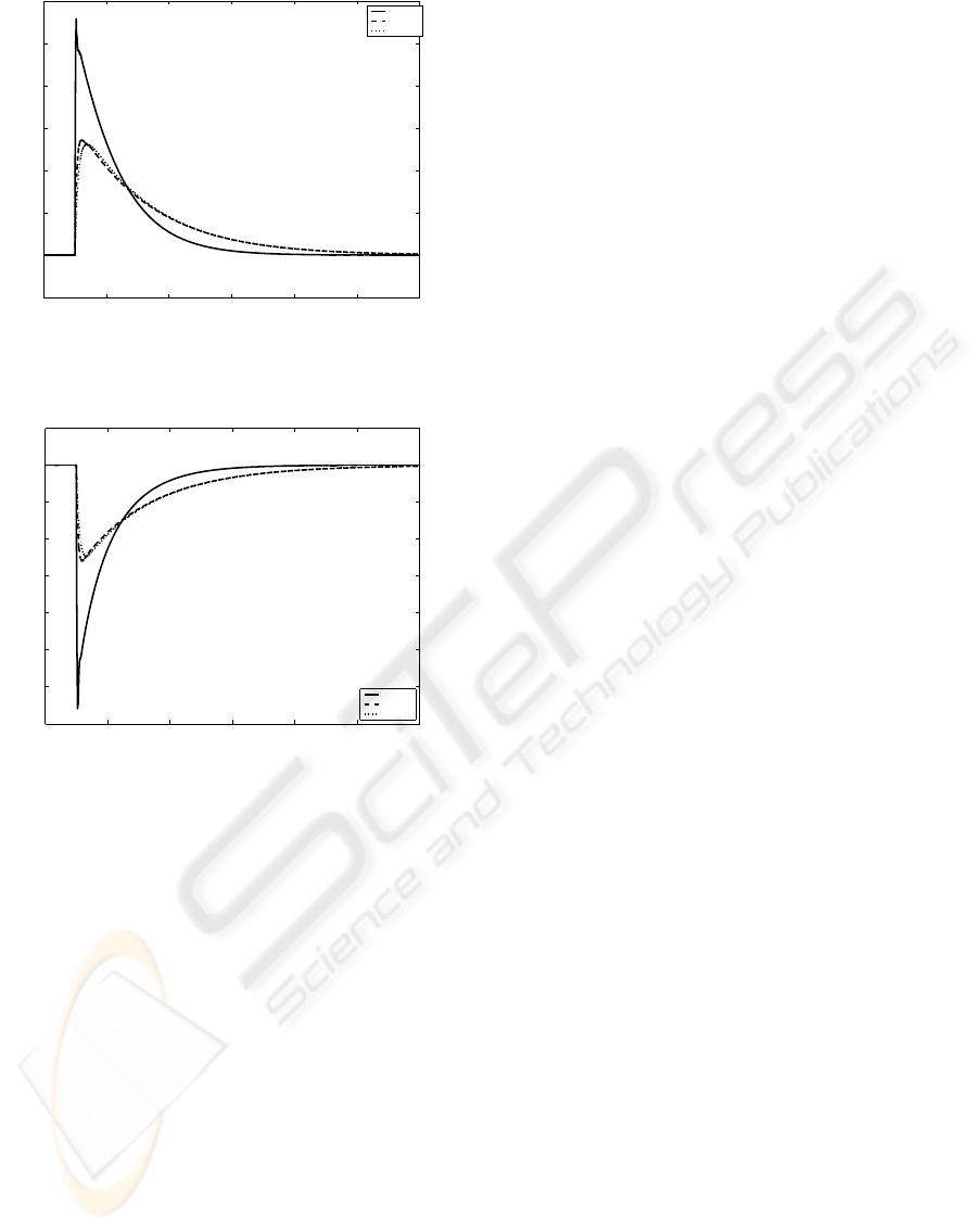
Fig. (1) shows the speed profile of the closed loop
systems of all three models for the load disturbance of
-10%. Fig. (2) shows the speed profile of the closed
loop systems of all models for the load disturbance of
+10%. It can be seen that in all cases the designed
robust controller is able to bring back the rotor speed
to the rated value.
6 CONCLUSION
In this paper, a design scheme of the control of in-
duction motor using fast output sampling control is
developed. The rotor speed is taken as output. The
output feedback control is applied at an appropriate
sampling rate to the nonlinear model of the plant.
As shown in plots, the proposed controller is able
to stabilize the speed around the operating points for
the change in load torque (T
L
) in spite of change in
plant model.
ROBUST CONTROL OF INDUCTION MOTOR USING FAST OUTPUT SAMPLING TECHNIQUE
29
0 5 10 15 20 25 30
1615
1620
1625
1630
1635
1640
1645
1650
time in sec.
speed in rpm
plant−1
plant−2
plant−3
Figure 1: Response of various models to -10% load dis-
tubance
0 5 10 15 20 25 30
1585
1590
1595
1600
1605
1610
1615
1620
1625
time in sec.
speed in rpm
plant−1
plant−2
plant−3
Figure 2: Response of various models to +10% load dis-
tubance
REFERENCES
Gahenet, P., Nemirovski, A., Laub, A. J. and Chilali, M.,
(1995), LMI Tool Box with for Matlab The Math
works Inc.: Natick MA.
Janson, P. L. and Lorenz, R. D., (1992), A physically in-
sightful approach to the design and accuracy assess-
ment of flux observers for field oriented induction ma-
chine drives EEE-IAS annual meeting record. ,570–
577.
Krause, P. C., Wasynczuk, O. and Sudhoff, S. D., (2002),
Analysis of Electric Machinery and Drive Systems
IEEE Press
Mohan N., (2000), Electric Drives : An Integrative Ap-
proach MNPERE Minneapolis.
Mohan N., (2001), Advanced Electric Drives : Analysis,
Control and modeling using Simulink MNPERE Min-
neapolis.
Sangwongwanich, S., Yonemoto, T., Furuhashi, T. and
Okuma, S., Design of sliding observer for robust es-
timation of rotor flux of induction motors Proceeding
of IPEC,Tokyo, 1235–1242..
Verghese, G. C. and Sanders, S. R., Observers for flux es-
timation in induction machine IEEE Trans. on Indus-
trial Electronics , 35(1):85–94.
Werner, H., (1996), Robust Control of a Laboratory Flight
Simulator by Non-dynamic Multi-rate Output Feed-
back, Proceeding of CDC , Kobe, Japan, 1575–1580.
Werner, H.,(1998), Multimodel robust control by fast output
sampling - LMI approach. Automatica, 34(2), 1625–
1630.
Werner, H., and Furuta, K., (1995), Simultaneous Stabi-
lization based on output measurement Kybernetika,
31, 395–411.
APPENDIX
A INDUCTION MOTOR
PARAMETERS
The following parameters are used for simulation of
the induction motor.
Power : 3 HP/2.4 KW
Voltage: 460 Volts (L-L, RMS)
Frequency: 60 Hz
Phases: 3
Full- Load Current: 4 A
Full- Load Speed: 1710 rpm
Full- Load Efficiency: 88.5%
Power Factor: 80.0%
No. of Poles: 4
slip=1.72%
Model Parameters Model-1 Mode-2 Mode-2
Rr 1.4Ω 46.2Ω 74Ω
Rs 1.2Ω 1.43Ω 1.77Ω
Xls 4.5Ω 6.72Ω 5.25Ω
Xlr 4.5Ω 6.72Ω 4.57Ω
Xm 142Ω 158Ω 139Ω
ICINCO 2005 - ROBOTICS AND AUTOMATION
30
