
VISUALLY SERVOING A GOUGH-STEWART PARALLEL ROBOT
ALLOWS FOR REDUCED AND LINEAR KINEMATIC
CALIBRATION
Nicolas Andreff and Philippe Martinet
LAboratoire des Sciences et Mat
´
eriaux pour l’Electronique et d’Automatique (LASMEA)
UMR 6602 CNRS-Universit
´
e Blaise Pascal
24 avenue des Landais, 63177 Aubire Cedex, France
Keywords:
parallel robot, visual servoing, redundant metrology, kinematic calibration.
Abstract:
This paper focuses on the benefits of using computer vision to control a Gough-Stewart parallel robot. Namely,
it is recalled that observing the legs of such a mechanism with a calibrated camera, thus following the redun-
dant metrology paradigm, simplifies the control law. Then, we prove in this paper that such a control law
depends on a reduced set of kinematic parameters (only those attached to the geometry of the robot base) and
that these parameters can be obtained by solving a linear system. Moreover, we show that the camera can
be calibrated without much experimental effort, simply using images of the robot itself. All this means that
setting up the control system consists only in placing the camera in front of the robot.
1 INTRODUCTION
Parallel mechanism are such that there exist several
kinematic chains (or legs) between their base and their
end-effector. Therefore, they may exhibit a better re-
peatability (Merlet, 2000) than serial mechanisms but
not a better accuracy (Wang and Masory, 1993), be-
cause of the large number of links and passive joints.
There can be two ways to compensate for the low ac-
curacy. The first way is to perform a kinematic cali-
bration of the mechanism and the second one is to use
a control law which is robust to calibration errors.
There exists a large amount of work on the control
of parallel mechanisms
1
. In the focus of attention,
Cartesian control is naturally achieved through the
use of the inverse Jacobian which transforms Carte-
sian velocities into joint velocities. It is noticeable
that the inverse Jacobian of parallel mechanisms does
not only depend on the joint configuration (as for ser-
ial mechanisms) but also on the end-effector pose.
Consequently, one needs to be able to estimate or
measure the latter. As far as we know, all the effort
has been put on the estimation of the end-effector
pose through the forward kinematic model and the
joint measurements. However, this yields much trou-
ble, related to the fact that in general, there is no
1
See http://www-sop.inria.fr/coprin/equipe/merlet for a
long list of references.
closed-form solution to the forward kinematic prob-
lem. Hence, one numerically inverts the inverse kine-
matic model, which is analytically defined for most of
the parallel mechanisms. However, it is known (Mer-
let, 1990; Husty, 1996) that this numerical inver-
sion requires high order polynomial root determina-
tion, with several possible solutions (up to 40 real
solutions for a Gough-Stewart platform (Dietmaier,
1998)). Much of the work is thus devoted to solv-
ing this problem accurately and in real-time (see for
instance (Zhao and Peng, 2000)), or to designing par-
allel mechanisms with analytical forward kinematic
model (Kim and Tsai, 2002; Gogu, 2004). One of
the promising paths lies in the use of the so-called
metrological redundancy (Baron and Angeles, 1998),
which simplifies the kinematic models by introducing
additional sensors into the mechanism and thus yields
easier control (Marquet, 2002).
Visual servoing (Espiau et al., 1992; Christensen
and Corke, 2003) is known to robustify the Carte-
sian control of serial and mobile robots, with tech-
niques ranging from position-based visual servoing
(PBVS) (Martinet et al., 1996) (when the pose mea-
surement is explicit) to image-based visual servoing
(IBVS) (Espiau et al., 1992) (when it is made implicit
by using only image measurements). Visual servo-
ing techniques are very effective since they close the
control loop on the vision sensor, which gives a di-
rect view of the Cartesian space. This yields a high
119
Andreff N. and Martinet P. (2005).
VISUALLY SERVOING A GOUGH-STEWART PARALLEL ROBOT ALLOWS FOR REDUCED AND LINEAR KINEMATIC CALIBRATION.
In Proceedings of the Second International Conference on Informatics in Control, Automation and Robotics - Robotics and Automation, pages 119-124
DOI: 10.5220/0001174301190124
Copyright
c
SciTePress
robustness to robot calibration errors. Indeed, these
errors only appear in a Jacobian matrix but not in the
regulated error.
Essentially, visual servoing techniques generate a
Cartesian desired velocity which is converted into
joint velocities by the robot inverse Jacobian. Hence,
one can translate such techniques to parallel mecha-
nisms as in (Koreichi et al., 1998; Kallio et al., 2000)
by observation of the robot end-effector and the use of
standard kinematic models. It is rather easier than in
the serial case, since the inverse Jacobian of a parallel
mechanism has a straightforward expression. More-
over, for parallel mechanisms, since the joint veloc-
ities are filtered through the inverse Jacobian, they
are admissible, in the sense that they do not gener-
ate internal forces. More precisely, this is only true
in the theoretical case. However, if the estimated in-
verse Jacobian used for control is close enough to the
actual one, the joint velocities will be closely admis-
sible, in the sense that they do not generate high in-
ternal forces.The only difficulty would come from the
dependency of the inverse Jacobian to the Cartesian
pose, which would need be estimated, but, as stated
above, vision can also do that (DeMenthon and Davis,
1992; Lavest et al., 1998) ! Notice that this point
pleads for PBVS rather than IBVS of parallel mecha-
nisms.
Nevertheless, the direct application of visual ser-
voing techniques assumes implicitly that the robot in-
verse Jacobian is given and that it is calibrated. There-
fore, modeling, identification and control have small
interaction with each other. Indeed, the model is usu-
ally defined for control using proprioceptive sensing
only and does not foresee the use of vision for con-
trol, then identification and control are defined with
the constraints imposed by the model. This is useful
for modularity but this might not be efficient in terms
of accuracy as well as of experimental set-up time.
On the opposite, instead of having identification
and control being driven by the initial modeling stage,
one could have a model taking into account the use of
vision for control and hence for identification. To do
so, a new way to use vision, which gathers the ad-
vantages of redundant metrology and of visual servo-
ing and avoids most of their drawbacks was presented
in (Andreff et al., 2005).
Indeed, adding redundant sensors is not always
technically feasible (think of a spherical joint) and al-
ways requires either that the sensors are foreseen at
design stage or that the mechanism is physically mod-
ified to install them after its building. Anyhow, there
are then additional calibration parameters in the kine-
matic model and one needs to estimate them in order
to convert redundant joint readings into a unit vector
expressed in the appropriate reference frame. More-
over, observing the end-effector of a parallel mecha-
nism by vision may be incompatible with its applica-
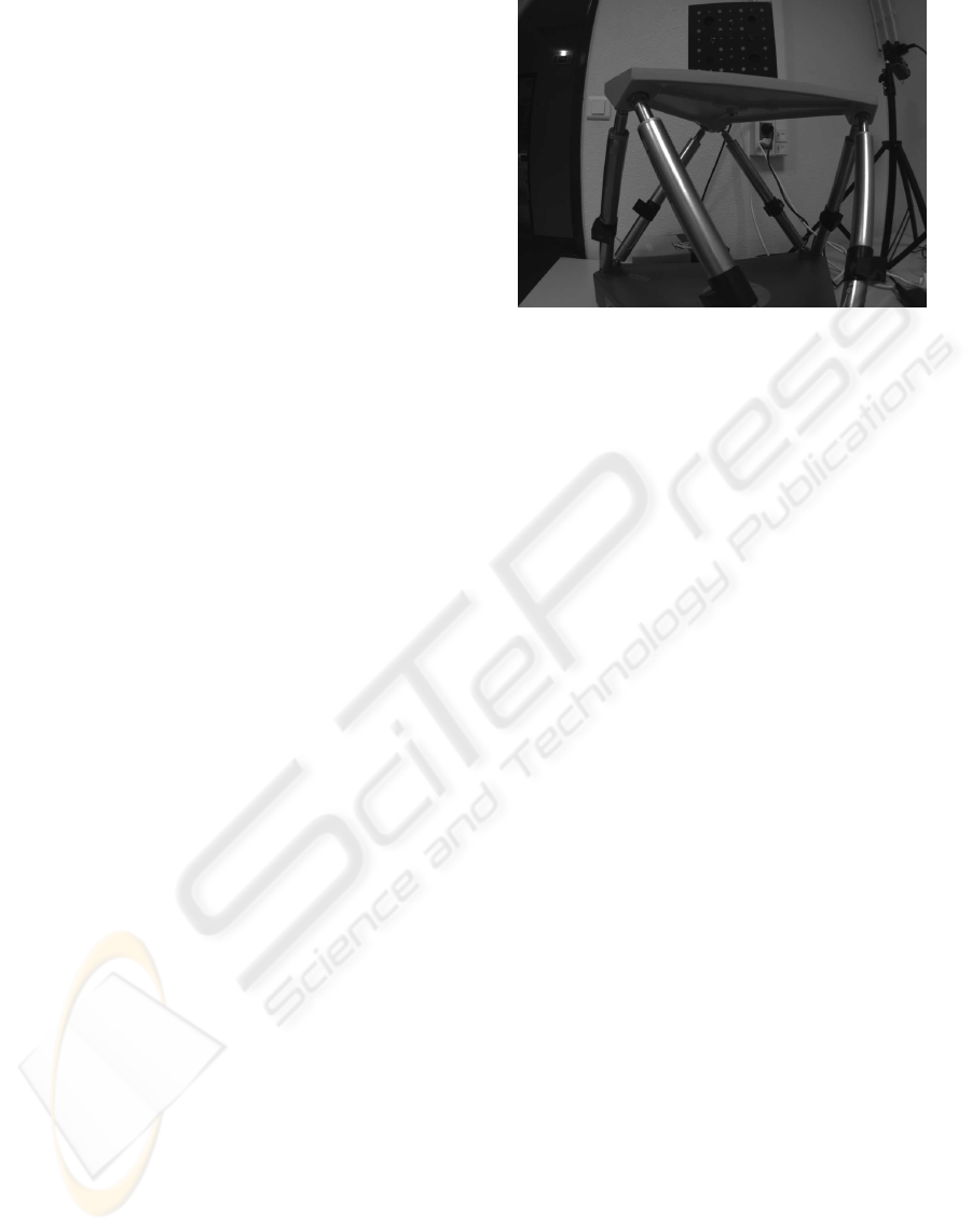
Figure 1: A Gough-Stewart platform observed by a camera
with short focal length.
tion. For instance, it is not wise to imagine observing
the end-effector of a machining tool. On the opposite,
it should not be a problem to observe the legs of the
mechanism, even in such extreme cases. Thereby one
would turn vision from an exteroceptive sensor to a
somewhat more proprioceptive sensor. This brings us
back to the redundant metrology paradigm.
With such an approach, the control is made easier
by measuring a major part of the robot inverse Jaco-
bian, reducing the number of kinematic parameters to
be identified. We will show in this paper that these
remaining parameters can be estimated by solving a
linear system.
The remainder of the paper is the following. Sec-
tion 2 recalls the vision-based control of the Gough-
Stewart robot. Section 3 discusses the actual choice of
vision for such a control. Section 4 presents the cali-
bration procedure for the whole system. Finally, sim-
ulation results and conclusion are given respectively
in section 5 and section 6.
2 VISION-BASED KINEMATICS
Consider the hexapod in Figure 1. It has 6 legs of
varying length q
i
, i ∈ 1..6, attached to the base by
spherical joints located in points A
i
and to the mov-
ing platform (end-effector) by spherical joints located
in points B
i
. The inverse kinematic model of such an
hexapod is given by
∀i ∈ 1..6, q
2
i
=
−−−→
A
i
B
i
T
−−−→
A
i
B
i
(1)
expressing that q
i
is the length of vector
−−−→
A
i
B
i
. This
model can be expressed in any Euclidean reference
frame. Hence, it can be expressed in the base frame
R
b
, in the end-effector frame R
e
or in the camera
frame R
c
. Hereafter, the camera reference frame will
be used and denoted by a left upper-script.
ICINCO 2005 - ROBOTICS AND AUTOMATION
120
According to (Andreff et al., 2005) and assuming
a calibrated camera, one can express the vision-based
kinematics of the hexapod expressed in the camera
frame:
q
i
c
u
i
=
c
R
e
e
B
i
+
c
t
e
−
c
B
i
(2)
˙
q =
c
J
inv
c
c
τ
c
(3)
with
c
J
inv
c
= −
c
u
T
1
(
c
A
1
×
c
u
1
)
T
.
.
.
.
.
.
c
u
T
6
(
c
A
6
×
c
u
6
)
T
(4)
where
c
τ
c
is the Cartesian velocity of the camera
frame, considered as attached to the base frame and
moving with respect to a fixed end-effector, expressed
in itself and
c
u
i
, i = 1..6 are the unit vectors giving
the pointing direction of each leg in the camera frame.
Then, one can derive a control law of the form:
e
i
=
c
u
i
×
c
u
d
i
(5)
E = (e
T
1
, ..., e
T
6
)
T
(6)
P(
c
u
i
) =
I
3
−
c
u
i
c
u
T
i
(7)
M
T
i
= P(
c
u
i
) [
I
3
−[
c
A
i
+ q
i
c
u
i
]
×
] (8)
N
T
i
=
1
q
i
[
c
u
d
i
]
×
M
T
i
(9)
N
T
= (N
1
, ..., N
6
)
T
(10)
˙
q = −λ
[c
J
inv
c
d
N
T
+
diag(q)E (11)
where the hat means that only an estimate can be used
and []
×
denotes the antisymmetric matrix associated
to the cross-product.
3 DISCUSSION
Here, the above control is discussed, with explicit re-
gard to the sensing problem. Indeed, it does not ab-
solutely imply that computer vision should be used
for that.
3.1 Why vision should be used
rather than joint sensors
There are three manners to measure or estimate the
u
i
’s. The first one, which we discard of course im-
mediately, is to estimate the end-effector pose with
respect to the base by numerical inversion of the in-
verse kinematic model and then use (2) to obtain u
i
.
The second manner is to place joint sensors in the
A
i
’s, so that they would deliver the pointing direc-
tion of the leg. This manner is valid since the u
i
’s
would be measured and not estimated through a del-
icate numerical procedure as above. Nevertheless, it
is, in our opinion, still not the correct manner. Indeed,
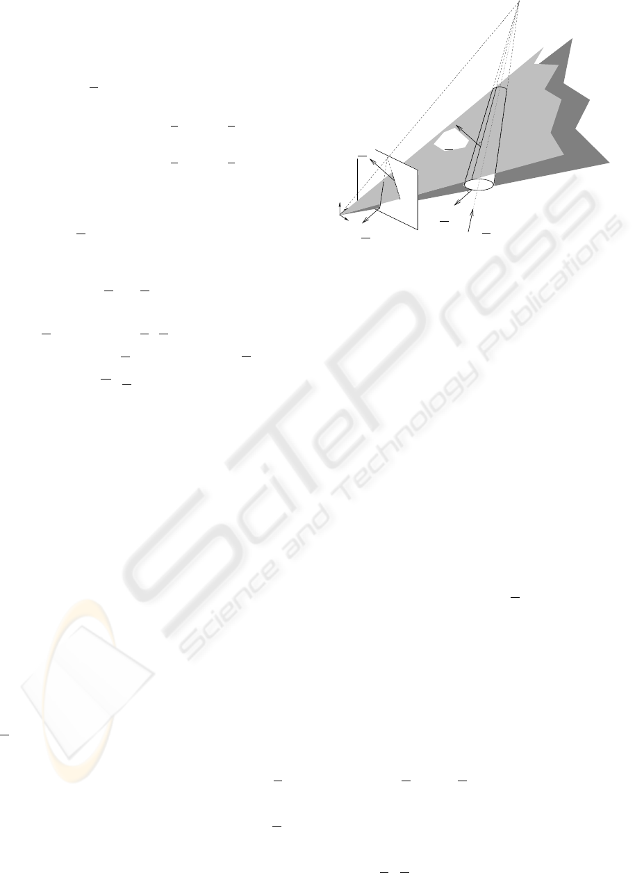
c
h
e
1
c
h
e
1
c
h
e
2
c
h
e
2
c
u
Figure 2: Projection of a cylinder in the image.
a joint sensor delivers a value expressed in its own ref-
erence frame. To convert this value in the base frame
would require either an extremely accurate assembly
procedure or the identification of the relative orien-
tation of each joint sensor frame with respect to the
base frame. Moreover, additional joint offsets would
need be identified.
Since the leading vector of a leg is essentially a
Cartesian feature, we chose to estimate it by vision.
Indeed, vision is an adequate tool for Cartesian sens-
ing, and, following (Renaud et al., 2004), if vision is
also chosen for calibration, this does not add extra cal-
ibration parameter. It will even be shown in Section 4
that using vision reduces the parameter set needed for
control.
3.2 Cylindrical leg observation
Now the problem is to recover
c
u
i
from the leg ob-
servation. It may be somehow tedious, although
certainly feasible, in the case of an arbitrary shape.
Hopefully, for mechanical reasons such as rigidity,
most of the parallel mechanisms are not only designed
with slim and rectilinear legs, but, even better, with
cylindrical shapes.
Except in the degenerated case where the projec-
tion center lies on the cylinder axis, the visual edge of
a cylinder is a straight line (Figure 2). Consequently,
it can be represented by its Binormalized Pl
¨
ucker co-
ordinates (Andreff et al., 2002) in the camera frame.
Let us note
c
h
e
1
and
c
h
e
2
the image projections of
the two edges of a cylinder, that can be tracked us-
ing the results in (Marchand and Chaumette, 2005).
These two vectors are oriented so that they point from
the cylinder revolution axis outwards. Then, their ex-
pression is related to the Binormalized Pl
¨
ucker Coor-
dinates (
c
u
,
c
h,
c
h) of the cylinder axis (see Figure 3)
VISUALLY SERVOING A GOUGH-STEWART PARALLEL ROBOT ALLOWS FOR REDUCED AND LINEAR
KINEMATIC CALIBRATION
121
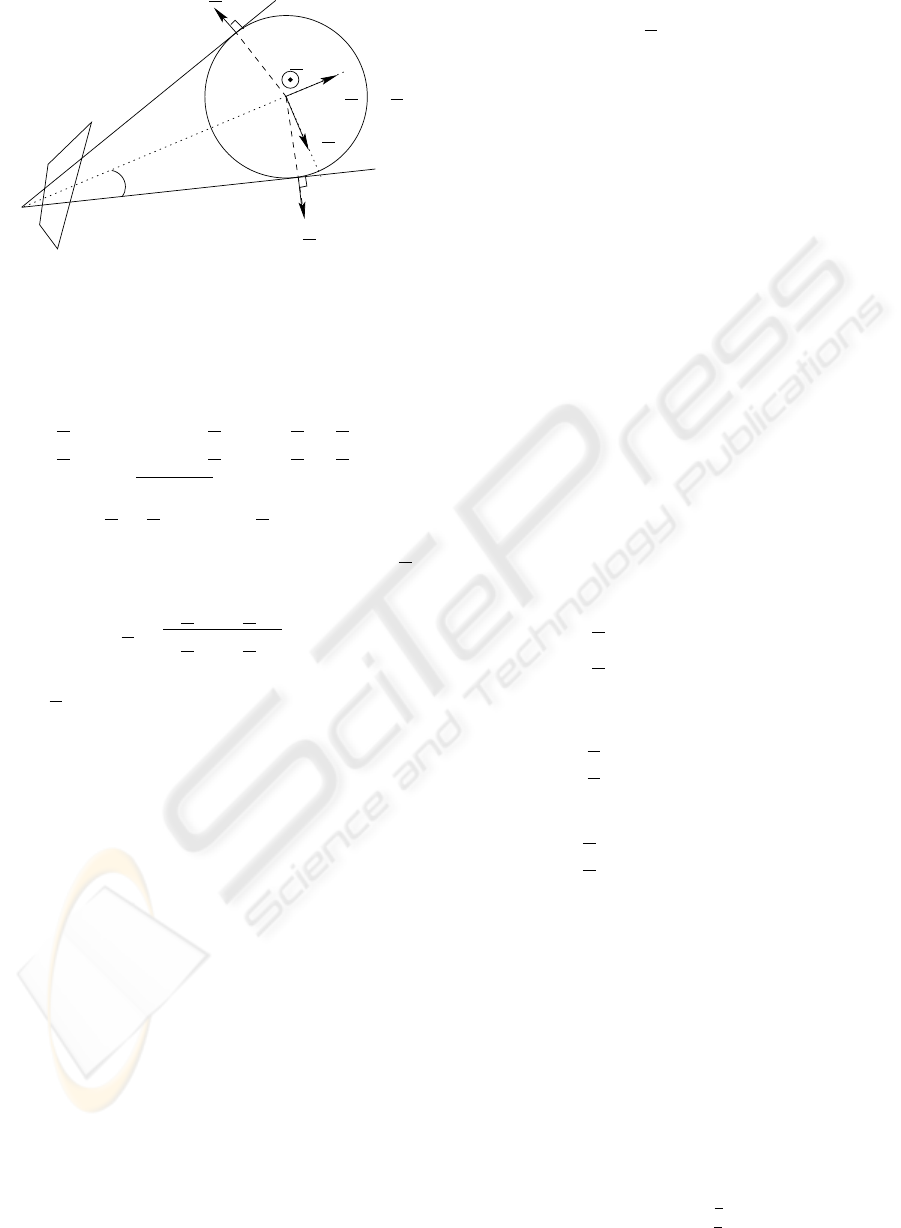
image plane
A
c
u
c
h
c
u
×
c
h
c
h
R
θ
c
h
e
1
c
h
e
2
Figure 3: Construction of the visual edges of a cylinder: the
cylinder is viewed from the top.
by
c
h
e
1
= −cos θ
c
h
− sin θ
c
u ×
c
h (12)
c
h
e
2
= + cos θ
c
h
− sin θ
c
u ×
c
h (13)
where cos θ =
√
c
h
2
− R
2
/
c
h and sin θ = R/
c
h,
c
h = k
c
A ×
c
u
k,
c
h = (
c
A ×
c
u)/
c
h and R is the
cylinder radius.
Then, it is easy to show that the leading vector
c
u
of the cylinder axis, expressed in the camera frame,
writes
c
u
=
c
h
e
1
×
c
h
e
2
k
c
h
e
1
×
c
h
e
2
k
(14)
Notice that the geometric interpretation of this result
is that
c
u
is, up to a scale factor, the vanishing point
of the two image edges, i.e. their intersection point in
the image.
4 VISION-BASED CALIBRATION
As stated earlier in this paper, the vision-based con-
trol (2)-(11) relies on the use of a calibrated camera
and on some kinematic parameters.
The classical approach for calibrating a camera is
to use a calibration grid made of points (Brown, 1971;
Tsai, 1986; Faugeras and Toscani, 1987; Lavest et al.,
1998). However, in the present case, it is more per-
tinent to use the method proposed in (Devernay and
Faugeras, 2001). Indeed, this method is based on the
observation of a set of lines, without any assumption
on their 3D structure. As can be seen in Figure 1,
there are plenty of lines in the images observed by
a camera placed in front of a Gough-Stewart parallel
robot. Hence, the camera can be calibrated on-line
without any experimental burden.
Now, the only kinematic parameters the control law
depends on are the attachment points of the legs onto
the base expressed in the camera frame (
c
A
i
) and on
the joint offsets. The latter appear in two places : un-
der the form
c
A
i
+ q
i
c
u
i
in (8) and as a gain in (9).
Considering the order of magnitude of
c
A
i
and q
i
,
one can neglect small errors on the joint offsets in (8).
Moreover, since the joints are prismatic it is easy to
measure their offsets manually with a millimetric ac-
curacy. This is also highly sufficient to ensure that the
gain in (9) is accurate enough. This means that, as far
as control is concerned, one only needs to identify the
attachment points onto the base, but there is no need
for identifying the other usual kinematic parameters:
attachment points onto the mobile platform and joint
offsets.
In (Renaud et al., 2004), a calibration procedure
was proposed, using legs observation, where, in a
first step, the points A
i
were estimated in the cam-
era frame, then in a second step were expressed in the
base frame, and finally the others kinematic parame-
ters where deduced. Essentially, only the first step of
this procedure is needed.
This step is reformulated here in a more elegant
way, using the Binormalized Pl
¨
ucker Coordinates of
the cylinder edges (12), and minimizing an image-
based criterion.
Assuming that the attachment point A
i
is lying on
the revolution axis of the leg and referring again to
Figure 3, one obtains, for any leg i and robot configu-
ration j,
c
h
e
1
i,j
T
c
A
i
= −R (15)
c
h
e
2
i,j
T
c
A
i
= −R (16)
Stacking such relations for n
c
robot configurations
yields the following linear system
c
h
e
1
i,1
T
c
h
e
2
i,1
T
.
.
.
c
h
e
1
i,n
c
T
c
h
e
2
i,n
c
T
c
A
i
=
−R
−R
.
.
.
−R
−R
(17)
which has a unique least-square solution if there are
at least two configurations with different leg orienta-
tions.
The calibration procedure is hence reduced to a
strict minimum. To improve its numerical efficiency,
one should only take care to use robot configurations
with the larger angles between each leg orientation.
However, since the
c
A
i
only appear in the interaction
matrix, they do not require a very accurate estimation.
5 RESULTS
A commercial DeltaLab hexapod was simulated,
such that
b
A
2k
= R
b
cos(k
π
3
+α)
sin(k
π
3
+α)
0
,
b
A
2k+1
=
ICINCO 2005 - ROBOTICS AND AUTOMATION
122
0 50 100 150 200 250 300 350 400 450 500
0
0.05
0.1
0.15
0.2
0.25
0.3
0.35
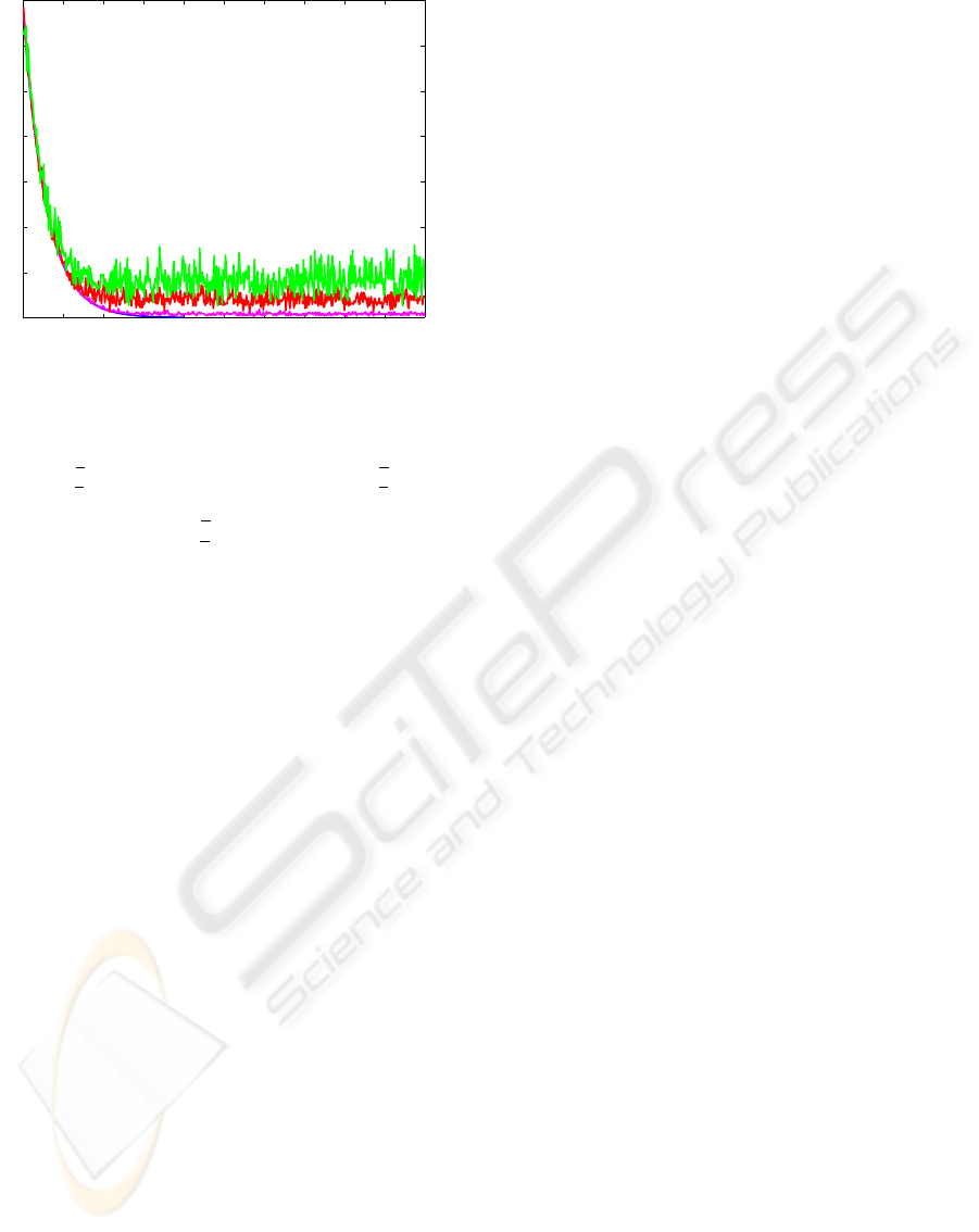
Figure 4: Robustness to noise : sum of squares of the errors
E
T
E with a noise amplitude of 0 deg, 0.01 deg, 0.05 deg
and 0.1 deg.
R
b
cos(k
π
3
−α)
sin(k
π
3
−α)
0
,
e
B
2k
= R
e
cos(k
π
3
+β)
sin(k
π
3
+β)
0
,
e
B
2k+1
= R
e
cos(k
π
3
−β)
sin(k
π
3
−β)
0
, k ∈ {0, 1, 2} with
R
b
= 270mm, α = 4.25
◦
, R
e
= 195mm, β =
5.885
◦
and the legs range are [345mm, 485mm].
5.1 Image noise
It is not immediate to model realistically the effect of
image noise on detecting the visual edges of a cylin-
der. One can imagine to use the (ρ, θ) representation
of an image line and to add noise to these two compo-
nents. However, it is not certain that the two noise
components are uncorrelated. Alternately, one can
also determine the virtual intersections of the visual
edge with the image border and to add noise to these
intersections (Bartoli and Sturm, 2004).
An alternative model is presented here, which takes
advantage of the fact that an image line is essentially
a unit vector. Thus, image noise will necessary result
into a rotation of this unit vector. Consequently, one
needs to define a random rotation matrix, that is to
say a rotation axis and a positive rotation angle. Pre-
liminary tests showed that simply taking this axis as
a uniformly distributed unit vector and this angle as a
uniformly distributed positive scalar gives a realistic
behavior.
This noise model has for advantages that it is easy
to implement, it does not depend on the simulated im-
age size, and is parametered by a single scalar (i.e. the
maximal amplitude of the rotation angle).
To give an idea of how to choose this maximal am-
plitude, an error of about ± 1 pixel on the extremities
of a 300 pixel-long line segment yields a rotation an-
gle of approximately 0.05 degree.
5.2 Calibration validation
In order to quantify the calibration procedure, the sim-
ulated robot was calibrated by moving it into its 64 ex-
tremal configurations (i.e. each leg joint is extended
to its lower limit then to its upper limit). In each con-
figuration, the visual edges of each leg were generated
from the inverse kinematic model and added noise as
described above, with a maximal amplitude of 0.05
degree. This calibration procedure was repeated 100
times. As a result, the median error on each attach-
ment point is less than 1 mm.
5.3 Realistic simulation
Now, a more realistic simulation is presented where
the calibration is first performed using the 64 extremal
configurations, then control is launched using the cal-
ibrated values. Noise is added as above during image
detection, with amplitudes of 0.01, 0.05 and 0.1 de-
gree.
It is noticeable that the calibration errors (in terms
of maximal error on each of the component of each
attachment point) is respectively of 0.5, 1.4 and 10
mm.
Graphically (Figure 4), the sum of the errors on
each leg E
T
E still decreases. Additionally, the me-
dian positioning error of the convergence tails in Fig-
ure 4 are respectively 0.1, 0.6 and 1.1 mm while the
maximal error are 0.6, 1.9 and 3 mm.
Hence, the overall calibration-control process
seems rather robust to image measurement errors.
6 CONCLUSION
A fundamentally novel approach was proposed
in (Andreff et al., 2005) for controlling a parallel
mechanism using vision as a redundant sensor, adding
a proprioceptive nature to the usual exteroceptive na-
ture of vision. The present paper shows that such a
method not only simplifies the control law, but also
reduces the experimental effort.
Indeed, on the opposite to standard Cartesian con-
trol, no numerical inversion of the inverse kinematic
model is required. Moreover, the kinematic parameter
set which is effectively used during vision-based con-
trol is smaller than the one used for Cartesian control.
Additionally, the kinematic calibration is turned lin-
ear with the vision-based approach.
From a practical point of view, setting-up such a
control is made easier than any other ones. Indeed,
on the opposite to most of the visual servoing ap-
proaches, there is no need to mount a visual target
onto the robot end-effector, since the visual targets are
the very robot legs. As far as calibration is concerned
VISUALLY SERVOING A GOUGH-STEWART PARALLEL ROBOT ALLOWS FOR REDUCED AND LINEAR
KINEMATIC CALIBRATION
123

again, the calibration of the camera can be done with
the same observation, as well as the kinematic cali-
bration, which does not require any more any specific
set-up.
Of course, all these benefits can only be obtained
to a higher cost in software integration and devel-
opment, which is not completely terminated at the
present time, preventing us from showing experimen-
tal results.
ACKNOWLEDGMENT
This study was jointly funded by CPER Auvergne
2003-2005 program and by the CNRS-ROBEA pro-
gram through the MP2 project.
REFERENCES
Andreff, N., Espiau, B., and Horaud, R. (2002). Visual ser-
voing from lines. Int. Journal of Robotics Research,
21(8):679–700.
Andreff, N., Marchadier, A., and Martinet, P. (2005).
Vision-based control of a Gough-Stewart parallel
mechanism using legs observation. In Proc. Int. Conf.
Robotics and Automation (ICRA’05), pages 2546–
2551, Barcelona, Spain.
Baron, L. and Angeles, J. (1998). The on-line direct kine-
matics of parallel manipulators under joint-sensor re-
dundancy. In Advances in Robot Kinematics, pages
126–137.
Bartoli, A. and Sturm, P. (2004). The 3d line motion matrix
and alignement of line reconstructions. Int. Journal of
Computer Vision, 57(3):159–178.
Brown, D. (1971). Close-range camera calibration. Pho-
togrammetric Engineering, 8(37):855–866.
Christensen, H. and Corke, P., editors (2003). Int. Journal of
Robotics Research – Special Issue on Visual Servoing,
volume 22.
DeMenthon, D. and Davis, L. (1992). Model-based object
pose in 25 lines of code. Lecture Notes in Computer
Science, pages 335–343.
Devernay, F. and Faugeras, O. (2001). Straight lines have to
be straight. Machine Vision and Applications, 13:14–
24.
Dietmaier, P. (1998). The Stewart-Gough platform of gen-
eral geometry can have 40 real postures. In Lenar
ˇ
ci
ˇ
c,
J. and Husty, M. L., editors, Advances in Robot Kine-
matics: Analysis and Control, pages 1–10. Kluwer.
Espiau, B., Chaumette, F., and Rives, P. (1992). A New Ap-
proach To Visual Servoing in Robotics. IEEE Trans.
on Robotics and Automation, 8(3).
Faugeras, O. and Toscani, G. (Tokyo, japan, 1987). Camera
calibration for 3d computer vision. In International
Conference on Computer Vision and Pattern Recogni-
tion (CVPR).
Gogu, G. (2004). Fully-isotropic T3R1-type parallel ma-
nipulator. In Lenar
ˇ
ci
ˇ
c, J. and Galletti, C., editors, On
Advances in Robot Kinematics, volume Kluwer Aca-
demic Publishers, pages 265–272.
Husty, M. (1996). An algorithm for solving the direct kine-
matics of general Gough-Stewart platforms. Mech.
Mach. Theory, 31(4):365–380.
Kallio, P., Zhou, Q., and Koivo, H. N. (2000). Three-
dimensional position control of a parallel microma-
nipulator using visual servoing. In Nelson, B. J.
and Breguet, J.-M., editors, Microrobotics and Mi-
croassembly II, Proceedings of SPIE, volume 4194,
pages 103–111.
Kim, H. and Tsai, L.-W. (2002). Evaluation of a Cartesian
parallel manipulator. In Lenar
ˇ
ci
ˇ
c, J. and Thomas, F.,
editors, Advances in Robot Kinematics: Theory and
Applications. Kluwer Academic Publishers.
Koreichi, M., Babaci, S., Chaumette, F., Fried, G., and
Pontnau, J. (1998). Visual servo control of a paral-
lel manipulator for assembly tasks. In 6th Int. Sympo-
sium on Intelligent Robotic Systems, SIRS’98, pages
109–116, Edimburg, Scotland.
Lavest, J., Viala, M., and Dhome, M. (1998). Do we really
need an accurate calibration pattern to achieve a reli-
able camera calibration. In Proceedings of ECCV98,
pages 158–174, Freiburg, Germany.
Marchand, E. and Chaumette, F. (2005). Feature track-
ing for visual servoing purposes. Robotics and Au-
tonomous Systems.
Marquet, F. (2002). Contribution
`
a l’
´
etude de l’apport de
la redondance en robotique parall
`
ele. PhD thesis,
LIRMM - Univ. Montpellier II.
Martinet, P., Gallice, J., and Khadraoui, D. (1996). Vision
based control law using 3d visual features. In Proc.
World Automation Congress, WAC’96, Robotics and
Manufacturing Systems, volume 3, pages 497–502,
Montpellier, France.
Merlet, J.-P. (1990). An algorithm for the forward kinemat-
ics of general 6 d.o.f. parallel manipulators. Technical
Report 1331, INRIA.
Merlet, J.-P. (2000). Parallel robots. Kluwer Academic
Publishers.
Renaud, P., Andreff, N., Gogu, G., and Martinet, P. (2004).
On vision-based kinematic calibration of a Stewart-
Gough platform. In 11th World Congress in Mech-
anism and Machine Science (IFToMM2003), pages
1906–1911, Tianjin, China.
Tsai, R. (Miami, UsA, 1986). An efficient and accurate
calibration technique for 3d machine vision. In Inter-
national Conference on Computer Vision and Pattern
Recognition (CVPR), pages pp 364–374.
Wang, J. and Masory, O. (1993). On the accuracy of a Stew-
art platform - Part I : The effect of manufacturing tol-
erances. In Proc. ICRA93, pages 114–120.
Zhao, X. and Peng, S. (2000). Direct displacement analysis
of parallel manipulators. Journal of Robotics Systems,
17(6):341–345.
ICINCO 2005 - ROBOTICS AND AUTOMATION
124
