
ROBUST ILC DESIGN USING MÖBIUS TRANSFORMATIONS
C. T. Freeman, P. L. Lewin and E. Rogers
University of Southampton
School of Electronics and Computer Science, University Road, Southampton, SO17 1BJ, United Kingdom
Keywords:
Learning control, non-minimum phase systems, optimisation.
Abstract:
In this paper a general ILC algorithm is examined and it is found that the filters involved can be selected to
satisfy frequency-wise uncertainty limits on the plant model. The probability of the plant model being at a
given point in the uncertainty space is specified, and the filters are then chosen to maximise the convergence
rate that can be expected in practice. The magnitude of the change in input over successive trials and the
residual error have also been incorporated into the cost function. Experimental results are presented using a
non-minimum phase test facility to show the effectiveness of the design method.
1 INTRODUCTION
Iterative Learning Control (ILC) is a control method
that is applicable to systems which perform the same
action repeatedly. Operating in this way it is able to
use past control information such as input signals and
tracking errors in the construction of the present con-
trol action. This sets ILC apart from most other con-
trol techniques and has allowed it to provide improved
performance with reduced knowledge of the plant
when compared with other control approaches. A lit-
erature survey of ILC can be found in (Moore, 1998)
and there exist textbooks on the subject (Moore, 1993;
Bien and Xu, 1998). One such ILC update law is
given by
u
k+1
= F (z)u
k
+ S(z)e
k
(1)
where e
k
= y
d
− y
k
and F (z) and S(z) are filters
which may be non-causal. This has been analysed in
the frequency-domain in, for example, (Norrlöf and
Gunnarsson, 1999) and (Norrlöf, 2000). Conversion
of (1) to the frequency-domain using the sampling pe-
riod, T
s
, gives
U
k+1
= F (e
jωT
s
)U
k
+ S(e
jωT
s
)E
k
(2)
Let the uncertain plant be described by G(e
jωT
s
) =
G
0
(e
jωT
s
)U(e
jωT
s
) where U (e
jωT
s
) is a multiplica-
tive uncertainty and G
0
the nominal plant model. In
this case the error evolution is
E
k+1
=
F (e
jωT
s
) − S(e
jωT
s
)G
0
(e
jωT
s
)U(e
jωT
s
) E
k
+
1 − F (e
jωT
s
) Y
d
(3)
so that
F (e
jωT
s
) − S(e
jωT
s
)G
0
(e
jωT
s
)U(e
jωT
s
)
< 1
(4)
is a necessary condition for stability since, for each
frequency, (3) represents a state-space system in the
iteration domain having a state transition matrix with
eigenvalues less than 1. In particular, if F (e
jωT
s
) =
1 this becomes a necessary condition for monotonic
convergence which can be shown to be essentially a
sufficient condition as well (Longman, 2000). More
generally, the same argument means
F (e
jωT
s
) − S(e
jωT
s
)G
0
(e
jωT
s
)U(e
jωT
s
)
< l
(5)
is a sufficient condition for the eigenvalues of the state
transition matrix to be less than l, or a reduction of
1
l
in the magnitude of the error over consecutive cycles
if F (e
jωT
s
) = 1. To accommodate both these cases,
satisfying (5) will be said to produce a convergence
rate of
1
l
.
Remark 1 Adding a filter, T (z), on the (k + 1)
th
cy-
cle error to the algorithm given in (1) produces
u
k+1
= F (z)u
k
+ S(z)e
k
+ T (z)e
k+1
(6)
and we can then write
y
k+1
=
G(z)T (z)
1+G(z)T (z)
y
d
+
G(z)
1+G(z)T (z)
(F (z)u
k
+ S(z)e
k
)
(7)
141
T. Freeman C., L. Lewin P. and Rogers E. (2005).
ROBUST ILC DESIGN USING MÖBIUS TRANSFORMATIONS.
In Proceedings of the Second International Conference on Informatics in Control, Automation and Robotics, pages 141-146
DOI: 10.5220/0001172601410146
Copyright
c
SciTePress

to give
u
k+1
=
T (z)
1+G(z)T (z)
y
d
+
1
1+G(z)T (z)
(F (z)u
k
+ S(z)e
k
)
(8)
The substitutions ˆy
d
=
T (z)
S(z)
+ 1
y
d
and
ˆ
G(z) =
G(z)
1+G(z)T (z)
, or alternatively ˆy
d
=
1
S(z)
+
1
T (z)
y
d
and
ˆ
G(z) =
G(z)T (z)
1+G(z)T (z)
, allow this to be written as
(1). Any design method for S(z) and F (z) can there-
fore be implemented as (6) using these substitutions.
Any robustness properties, however, will only apply to
ˆ
G(z) instead of G(z).
2 DFT
An alternative expression for (2) is found by taking
the Discrete Fourier Transform (DFT) of both sides
of the update law (1) which results in
ˆu
k+1
=
ˆ
F ⊙ ˆu
k
+
ˆ
S ⊙ ˆe
k
(9)
which is possible since e
k
and u
k
are known prior to
the k + 1
th
trial. Here ⊙ denotes component-wise
multiplication and ˆu is the DFT of u. Similarly, the
DFT of (3) results in an alternative description
ˆe
k+1
= (
ˆ
F −
ˆ
G
0
⊙
ˆ
U ⊙
ˆ
S) ⊙ ˆe
k
+(I −
ˆ
F )⊙ ˆy
d
(10)
Note that now the design is conducted in the
frequency-domain, the designer can select each ele-
ment
ˆ
S
i
and
ˆ
F
i
individually and build the new in-
put u
k+1
using (9) combined with expressions for the
DFT and IDFT of a signal. Similar transparency can-
not be found in the time domain. Since (4) is a steady-
state requirement which assumes a reasonable tran-
sient response, the use of a steady-state update of the
input is not disadvantageous. It just remains to choose
the value of the filters S and F at every frequency.
3 APPROACH TO FILTER
DESIGN
By introducing the variable v = U (e
jωT
s
) it is possi-
ble to write (5) as
sup
ω ∈[0,2π]
|f(v)| < l (11)
where
f(v) = F (e
jωT
s
) − S(e
jωT
s
)G
0
(e
jωT
s
)v v ∈ C
(12)
Let the open disc of radius l centred at the origin,
and its boundary be defined as
D = {r e
jθ
| θ ∈ [−π π), r ∈ [0 l)},
δD = {le
jθ
| θ ∈ [−π π)}
(13)
so that the inverse function
f
−1
(v) =
F (e
jωT
s
) + v
S(e
jωT
s
)G
0
(e
jωT
s
)
v ∈ C (14)
applied to D gives the range of values taken by
U(e
jωT
s
) for (5) to be satisfied.
The domain and co-domain can be enlarged to
equal the extended complex plane
ˆ
C (Jones and
Singerman, 2004) which is the union of C and the
point at infinity; thus
ˆ
C = C ∪ {∞}. In this case
f
−1
(v) is an extended Möbius transformation when
ω and T
s
are fixed, and maps
•
ˆ
C one-one onto
ˆ
C
• generalised circles onto generalised circles
A generalised circle is defined as either a circle or an
extended line (see (Jones and Singerman, 2004) for
details).
It is therefore possible to apply f
−1
(v) to δD and
find the boundary of the region U(e
jωT
s
) must oc-
cupy to ensure a convergence rate of
1
l
, or monotonic
convergence if l ≤ 1. The image of a Möbius trans-
formation can be found by simply applying f
−1
(v) to
three points of δD and finding the unique generalised
circle which passes through the resulting points (see
(Jones and Singerman, 2004)). Since {±l, lj} ∈ δD,
f
−1
(+l) =
F (e
jωT
s
)+l
S(e
jωT
s
)G
0
(e
jωT
s
)
f
−1
(−l) =
F (e
jωT
s
)−l
S(e
jωT
s
)G
0
(e
jωT
s
)
f
−1
(lj) =
F (e
jωT
s
)+lj
S(e
jωT
s
)G
0
(e
jωT
s
)
(15)
belong to this extended circle. However a simpler
method involves noting that the inverse points of δD
are 0 and ∞ so that the inverse points of the image are
given by
f
−1
(0) =
F (e
jωT
s
)
S(e
jωT
s
)G
0
(e
jωT
s
)
, f
−1
(∞) = ∞
(16)
and the mapping has the form
z −
F (e
jωT
s
)
S(e
jωT
s
)G
0
(e
jωT
s
)
= k(e
jωT
s
) (17)
Since f
−1
(l) =
F (e
jωT
s
)+l
S(e
jωT
s
)G
0
(e
jωT
s
)
∈ δD then
F (e
jωT
s
) + l
S(e
jωT
s
)G
0
(e
jωT
s
)
−
F (e
jωT
s
)
S(e
jωT
s
)G
0
(e
jωT
s
)
= k(e
jωT
s
) =
l
|S(e
jωT
s
)G
0
(e
jωT
s
)|
(18)
which is the equation for a circle with centre, λ, and
radius, r, where
λ =
F (e
jωT
s
)
S(e
jωT
s
)G
0
(e
jωT
s
)
, r =
l
|S(e
jωT
s
)G
0
(e
jωT
s
)|
(19)
ICINCO 2005 - INTELLIGENT CONTROL SYSTEMS AND OPTIMIZATION
142
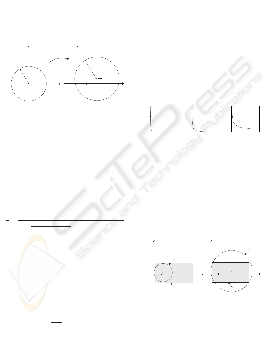
This circle can then be drawn for every frequency of
interest and hence the region U(e
jωT
s
) must occupy
in order to guarantee monotonic convergence. Note
that a Möbius transformation, t(z), maps a region R
in its domain to a region t(R), and the boundary of
R to the boundary of t(R). Figure 1 shows the ac-
tion of f
−1
(v) on δD and the region U(e
jωT
s
) must
occupy for a convergence rate of
1
l
. Any uncertainty
F
SG
Re
Im
1
Uncertaintyspace
SG
Re
Im
f (v)
-1
l
l
Figure 1: Geometry of uncertainty space
that is contained within the right-hand circle for all
frequencies will satisfy (5). At a general point, p, in
the uncertainty space we can equate the distance from
p to λ with r
p −
F (e
jωT
s
)
S(e
jωT
s
)G
0
(e
jωT
s
)
=
l
|S(e
jωT
s
)G
0
(e
jωT
s
)|
(20)
in order to find the convergence rate at that frequency
1
l
=
1
p −
F (e
jωT
s
)
S(e
jωT
s
)G
0
(e
jωT
s
)
|S(e
jωT
s
)G
0
(e
jωT
s
)|
=
1
|S(e
jωT
s
)G
0
(e
jωT
s
)p − F (e
jωT
s
)|
(21)
This provides a useful means of selecting S and F :
Let us choose to maximize the convergence rate that
can be expected given that the probability that the
plant is at the point p at a given frequency is known
or can be estimated. It will be assumed that this prob-
ability is symmetrical about the nominal value, that
is +1 in the uncertainty space. This is a situation
which is realistic given the methods of obtaining a
plant model commonly used in practice. In this case it
will be a function of the distance to the nominal plant
model which equals
1
|p−1|
in the uncertainty space.
The optimisation will therefore take the form
max
S,F
J(S, F ) (22)
with the cost function
J(S, F ) =
Z
A
1
p −
F
SG
0
|SG
0
|
P
1
|p − 1|
δp
=
1
|SG
0
|
Z
A
1
p −
F
SG
0
P
1
|p − 1|
δp
(23)
where P (·) is the probability that the plant is at p,
and A is a region of uncertainty over which P (·) is
valid. The frequency dependence of the filters has
been dropped for conciseness. Note that a small circle
around the singularity must be removed if the equa-
tion is solved numerically. Figure 2 shows three cases
using the probability function P (x) = x
−α
and α
equal to 2, 1 and 0.5. The probability function is able
0 0.5 1
0
5000
10000
x
P(x) = x
−2
0 0.5 1
0
50
100
x
P(x) = x
−1
0 0.5 1
0
5
10
x
P(x) = x
−0.5
Figure 2: Examples of P (x)
to shift focus between robustness and convergence
speed by varying the weighting of the optimisation.
In the first case P (x) is only large for x ≈ 0 so the
maximisation will lead to a solution which is tailored
to only values close to the nominal plant model. As α
is reduced it becomes more important to choose S so
that the whole of A has a value of l < 1. These cases
are shown in Figure 3. In a)
1
SG
≈ 1 to give a high
convergence rate for the nominal plant, whilst in b) it
is smaller but most of the region A has the property of
satisfying (5). This choice of P (x) produces the cost
Re
Im
1
1
SG
Re
Im
1
1
SG
a)
b)
f (1)
-1
A
A
f (1)
-1
Figure 3: Optimal solutions for a) α > 1 and b) α < 1
J(S, F ) =
1
|SG
0
|
Z
A
|p − 1|
α
p −
F
SG
0
δp (24)
ROBUST ILC DESIGN USING MÖBIUS TRANSFORMATIONS
143

and the values of S and F are found by solving
∂
∂S
J(S, F ) = 0 and
∂
∂F
J(S, F ) = 0 (25)
at each frequency and ensuring that it is a global max-
imum. If F is fixed at 1 then any solution, S
∗
which
solves (25), so that
dJ(S
∗
, 1)
dS
= 0 (26)
will also solve the optimisation using
J
S
F
=
|F |
|S||G
0
|
Z
A
|p − 1|
α
p −
F
SG
0
δp (27)
since only a substitution of variables has been applied.
S and F can assume any values as long as
S
F
= S
∗
.
If F is now fixed at
ˆ
F , the corresponding value of
ˆ
S
is
ˆ
F S
∗
. This must also solve the optimisation using
(24) as this is simply (27) multiplied by a constant.
Therefore it is enough to solve the optimisation using
(24) with F = 1 and simply substitute
ˆ
S =
ˆ
F S
∗
to obtain the solution for every other value of F . The
resulting cost is
ˆ
J = |
ˆ
F |J
∗
where J
∗
is the cost using
F = 1. In order to incorporate other considerations in
the cost, let us consider the change in input from one
trial to the next. Since this is given by
u
k+1
− u
k
= (F − 1)u
k
+ Se
k
(28)
which, with the repeated application of (3), becomes
u
k+1
− u
k
= S (F − SG
0
U)
k
e
0
+
S(1 − F )
k−1
X
i=0
(F − SG
0
U)
i
y
d
+ (F − 1)u
k
(29)
and the residual error is given by
e
k
= (F − SG
0
U)
k
e
0
+(1−F )
k−1
X
i=0
(F − SG
0
U)
i
y
d
(30)
It can be seen that reducing F from 1 therefore has
the effect of reducing the cost (24) with the compro-
mise of a likelihood of increased residual error and
input change. To tackle these effects directly for an
arbitrary e
0
and y
d
, it is required that each term in
(29) and (30) has a small modulus for each frequency
considered. Assuming that (4) is satisfied it remains
to reduce |S| and also the bound, λ, on the remaining
term which is given by
(1 − F )
P
k−1
i=0
(F − SG
0
U)
i
y
d
<
1−F
1−(F −SG
0
U)
= λ
(31)
This can be achieved using the mapping technique
that has already been described. Using this, we find
that at a point in the uncertainty space, p, the bound λ
equals
1 − F
SG
0
p +
1−F
SG
0
=
1
SG
0
1−F
p + 1
(32)
Therefore the functions Q(|S|
−1
) and
R
SG
0
1−F
p + 1
can be incorporated into the
cost to limit the upper bound of the residual error
and change in successive inputs. Since these are
dependent on the plant and choice of y
d
, they will be
neglected in order to maintain focus on the general
case.
3.1 Experimental Test Facility
The experimental non-minimum phase test-bed has
previously been used to evaluate a number of Repet-
itive Control and ILC schemes (see (Freeman et al.,
2005) for details) and consists of a rotary mechanical
system of inertias, dampers, torsional springs, a tim-
ing belt, pulleys and gears. An encoder records the
ouput shaft position and a standard squirrel cage in-
duction motor drives the load. The system has been
modelled using a LMS algorithm to fit a linear model
to a great number of frequency response test results.
The resulting continuous time plant transfer function
has thus been established as
G
0
(s) =
1.202(4 − s)
s(s + 9)(s
2
+ 12s + 56.25)
(33)
A PID loop around the plant is used in order to act as
a pre-stabiliser and provide greater stability. The PID
gains used are K
p
= 137, K
i
= 5 and K
d
= 3. The
resulting closed-loop system constitutes the system to
be controlled.
4 EXPERIMENTAL RESULTS
In polar co-ordinates let us define the region
A = {re
jθ
| θ ∈ [θ
m
θ
M
], r ∈ [r
m
r
M
]} (34)
in the uncertainty space over which the probabil-
ity function is valid. The parameters T = 6 and
n = 1024 are chosen for convenience to give fs =
1024/6. Let us solve the optimisation using (24) with
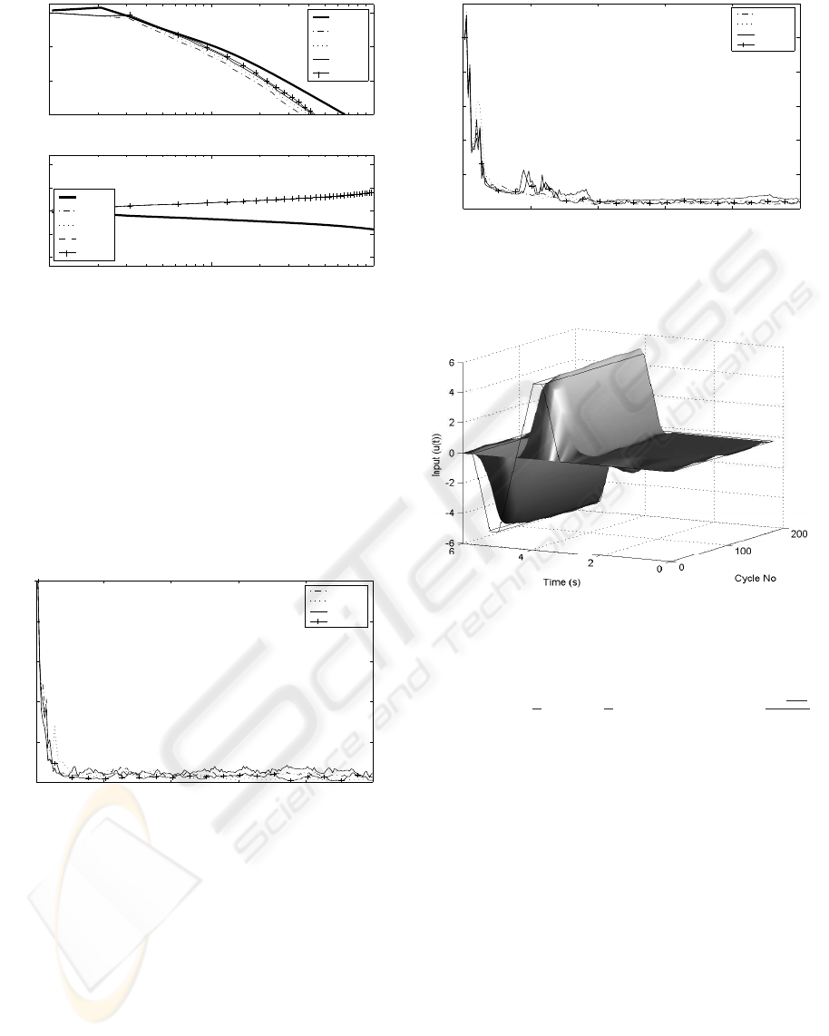
F = 1 and α = 0.2. Figure 4 shows a Bode plot of the
resulting S vectors when using θ
m
= −
π
6
, θ
M
=
π
6
,
r
m
= 0 and r
M
=
1+
T ω
2πλ
|G
0
|
2
with λ = 4, 6, 8, 10.
These have been chosen using previous experience of
the plant uncertainty. As λ increases, r
M
decreases,
which, in turn, increases the magnitude of S at each
frequency as the plant effectively becomes less un-
certain as A diminishes in size. Since θ
m
= −θ
M
,
ICINCO 2005 - INTELLIGENT CONTROL SYSTEMS AND OPTIMIZATION
144
10
0
10
1
10
2
−150
−100
−50
0
Gain (dB)
Frequency (rad/s)
10
0
10
1
10
2
−2000
−1000
0
1000
2000
Phase (degrees)
G
0
λ = 4
λ = 6
λ = 8
λ = 10
G
0
λ = 4
λ = 6
λ = 8
λ = 10
Figure 4: Bode plot using various r
M
functions and α =
0.2
A is symmetrical about the real axis which results in
∠S = −∠G
0
. Figure 5 shows error results using the
sinewave demand (shown in figure 11). The normal-
ized error ‘NE’ is the cumulative error incurred over
an iteration divided by the integral of the reference de-
mand. Data has been recorded over the course of 200
iterations. It can be seen that smaller λ values lead to
reduced fluctuations in the cycle error. Figure 6 shows
0 40 80 120 160 200
0
0.2
0.4
0.6
0.8
1
Cycle No.
NE
λ = 4
λ = 6
λ = 8
λ = 10
Figure 5: Cycle error for sinewave demand
error results using the sinewave demand (shown in
figure 7). Due to the higher frequencies present in
the demand, the convergence is slower and the resid-
ual error greater. Higher frequency properties of the
optimisation play a greater role and so the effect of
λ on the learning transients is more pronounced than
previously. The convergence of the output to the de-
mand is shown in figure 7 using λ = 6. The repeating
sequence demand is also drawn.
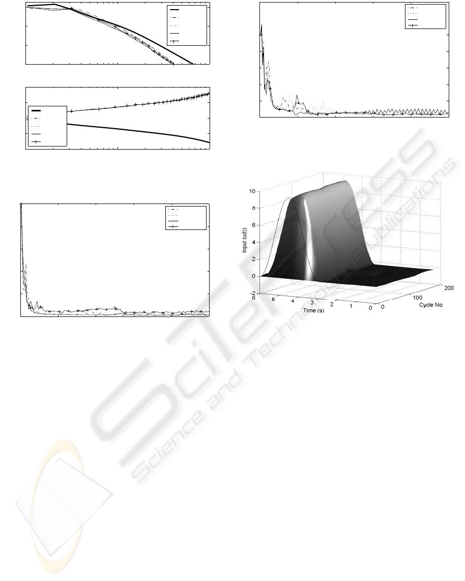
To investigate the effect of variation in α, the op-
timisation using (24) with F = 1 has again been
solved but using α = 0.1, 0.3, 0.5, 0.7. Figure 8
shows a Bode plot of the resulting S vectors when
0 40 80 120 160 200
0
0.2
0.4
0.6
0.8
1
Cycle No.
NE
λ = 4
λ = 6
λ = 8
λ = 10
Figure 6: Cycle error for repeating sequence demand
Figure 7: Output tracking using repeating sequence demand
and λ = 6
using θ
m
= −
π
6
, θ
M
=
π
6
, r
m
= 0 and r
M
=
1+
T ω
2πλ
|G
0
|
2
with λ = 6. As α increases in magnitude more em-
phasis is put on fast convergence for the nominal plant
and the gain is larger for a greater range of frequen-
cies. Figure 9 shows error results using the sinewave
demand and it can be seen that higher α values pro-
duce greater learning transients, and, ultimately, di-
vergence. They do, however, produce faster initial
convergence. Figure 10 shows error results using the
repeating sequence demand which confirm the previ-
ous findings. The convergence of the output to the
demand is shown in figure 11 using α = −0.5 and
the sinewave demand which is also shown.
5 FUTURE WORK
Since the uncertainty probability function can only be
an approximation, an obvious method to increase al-
gorithm robustness is to use additional plant data and
attempt to locate the plant model with greater accu-
ROBUST ILC DESIGN USING MÖBIUS TRANSFORMATIONS
145
10
0
10
1
10
2
−150
−100
−50
0
Gain (dB)
Frequency (rad/s)
10
0
10
1
10
2
−1000
−500
0
500
1000
Phase (degrees)
G
0
α =−0.7
α =−0.3
α =−0.1
α =−0.5
G
0
α =−0.7
α =−0.3
α = −0.1
α =−0.5
Figure 8: Bode plot using various α, λ = 6
0 40 80 120 160 200
0
0.2
0.4
0.6
0.8
1
Cycle No.
NE
α = −0.1
α = −0.3
α = −0.5
α = −0.7
Figure 9: Cycle error for sinewave demand
racy as the iterations progress. At the same time, the
added confidence in the nominal plant value could al-
low the focus of the optimisation to be shifted from
robustness to convergence speed. This would be
achieved by adaptively varying the probability func-
tion from trial to trial and seeking to reduce the radii
of circles corresponding to convergence rates for each
frequency around the nominal plant model. This use
of adaptive parameter tuning will be investigated in
conjunction with different plant models to confirm its
effectiveness.
The terms that have been derived in order to tackle
the magnitude of the residual error and the change in
input over successive cycles must be added to the cost
function and experiments conducted to examine their
performance in practice.
REFERENCES
Bien, Z. and Xu, J. (1998). Iterative Learning Con-
trol, Analysis, Design, Integration and Applications.
Kluwer Academic Publishers.
0 40 80 120 160 200
0
0.2
0.4
0.6
0.8
1
Cycle No.
NE
α = −0.1
α = −0.3
α = −0.5
α = −0.7
Figure 10: Cycle error for repeating sequence demand
Figure 11: Output tracking using sinewave demand and
α = 0.5
Freeman, C. T., Lewin, P. L., and Rogers, E. (2005). Exper-
imental evaluation of iterative control algorithms for
non-minimum phase plants. International Journal of
Control, 78(11):806–826.
Jones, G. A. and Singerman, D. (2004). Complex Func-
tions: An Algebraic and Geometric Viewpoint. Cam-
bridge University Press.
Longman, R. W. (2000). Iterative learning control and
repetitive control for engineering practice. Interna-
tional Journal of Control, 73(10):930–954.
Moore, K. L. (1993). Iterative Learning Control for Deter-
ministic Systems. Springer-Verlag.
Moore, K. L. (1998). Iterative learning control - an expos-
itory overview. Applied and Computational Controls,
Signal Processing and Circuits, 1(1):151 – 214.
Norrlöf, M. (2000). Comparative study on first and second
order ilc- frequency domain analysis and experiments.
In Proceedings of the 39th Conference on Decision
and Control, pages 3415–3420.
Norrlöf, M. and Gunnarsson, S. (1999). A frequency do-
main analysis of a second order iterative learning con-
trol algorithm. In Proceedings of the 38th Conference
on Decision and Control, pages 1587–1592.
ICINCO 2005 - INTELLIGENT CONTROL SYSTEMS AND OPTIMIZATION
146
