
EVOLUTIONARY COMPUTATION FOR DISCRETE AND
CONTINUOUS TIME OPTIMAL CONTROL PROBLEMS
Yechiel Crispin
Department of Aerospace Engineering
Embry-Riddle University
Daytona Beach, FL 32114
Keywords:
Optimal Control, Rocket Dynamics, Goddard’s Problem, Evolutionary Computation, Genetic Algorithms.
Abstract:
Nonlinear discrete time and continuous time optimal control problems with terminal constraints are solved
using a new evolutionary approach which seeks the control history directly by evolutionary computation.
Unlike methods that use the first order necessary conditions to determine the optimum, the main advantage of
the present method is that it does not require the development of a Hamiltonian formulation and consequently,
it eliminates the requirement to solve the adjoint problem which usually leads to a difficult two-point boundary
value problem. The method is verified on two benchmark problems. The first problem is the discrete time
velocity direction programming problem with the effects of gravity, thrust and drag and a terminal constraint
on the final vertical position. The second problem is a continuous time optimal control problem in rocket
dynamics, the Goddard’s problem. The solutions of both problems compared favorably with published results
based on gradient methods.
1 INTRODUCTION
An optimal control problem consists of finding the
time histories of the controls and the state variables
such as to maximize an integral performance index
over a finite period of time, subject to dynamical con-
straints in the form of a system of ordinary differential
equations (Bryson, 1975). In a discrete-time optimal
control problem, the time period is divided into a fi-
nite number of time intervals of equal duration ∆T .
The controls are kept constant over each time inter-
val. This results in a considerable simplification of the
continuous time problem, since the ordinary differen-
tial equations can be reduced to difference equations
and the integral performance index can be reduced to
a finite sum over the discrete time counter (Bryson,
1999). In some problems, additional constraints may
be prescribed on the final states of the system.
Modern methods for solving the optimal control
problem are extensions of the classical methods of the
calculus of variations (Fox, 1950). These methods are
known as indirect methods and are based on the max-
imum principle of Pontryagin, which is a statement of
the first order necessary conditions for optimality, and
results in a two-point boundary value problem (TP-
BVP) for the state and adjoint variables (L.S. Pon-
tryagin and Mishchenko, 1962).
It has been known, however, that the TPBVP is
much more difficult to solve than the initial value
problem (IVP). As a consequence, a second class of
solutions, known as the direct method has evolved.
For example, attempts have been made to recast the
original dynamic optimization problem as a static
optimization problem by direct transcription (Betts,
2001) or some other discretisation method, eventually
reformulating the original problem as a nonlinear pro-
gramming (NLP) problem. This is often achieved by
parameterisation of the state variables or the controls,
or both. The original differential equations or differ-
ence equations are reduced to algebraic equality con-
straints. A significant advantage of this method is that
the Hamiltonian formulation is completely avoided,
which can be advantageous to practicing engineers
who have not been exposed to the theoretical frame-
work of optimal control. However, there are some
problems with this approach. First, it might result in a
large scale NLP problem which might suffer from nu-
merical stability and convergence problems and might
require excessive computing time. Also, the para-
meterisation might introduce spurious local minima
which are not present in the original problem.
With the advent of computing power and the
45
Crispin Y. (2005).
EVOLUTIONARY COMPUTATION FOR DISCRETE AND CONTINUOUS TIME OPTIMAL CONTROL PROBLEMS.
In Proceedings of the Second International Conference on Informatics in Control, Automation and Robotics, pages 45-54
DOI: 10.5220/0001171200450054
Copyright
c
SciTePress

progress made in methods that are based on op-
timization analogies from nature, it became pos-
sible to achieve a remedy to some of the above
mentioned disadvantages through the use of global
methods of optimization. These include stochas-
tic methods, such as simulated annealing (Laarhoven
and Aarts, 1989), (Kirkpatrick and Vecchi, 1983)
and evolutionary computation methods (Fogel, 1998),
(Schwefel, 1995) such as genetic algorithms (GAs)
(Michalewicz, 1992), see also (Z. Michalewicz and
Krawczyk, 1992) for an interesting treatment of the
linear discrete-time problem.
Genetic algorithms provide a powerful mechanism
towards a global search for the optimum, but in many
cases, the convergence is very slow. However, as will
be shown in this paper, if the GA is supplemented
by problem specific heuristics, the convergence can
be accelerated significantly. It is well known that
GAs are based on a guided random search through
the genetic operators and evolution by artificial se-
lection. This process is inherently very slow, be-
cause the search space is very large and evolution pro-
gresses step by step, exploring many regions with so-
lutions of low fitness. However, it is often possible to
guide the search further, by incorporating qualitative
knowledge about potential good solutions. In many
problems, this might involve simple heuristics, which
when combined with the genetic search, provide a
powerful tool for finding the optimum very quickly.
The purpose of the present work is to incorporate
problem specific heuristic arguments, which when
combined with a modified hybrid GA, can solve
the discrete-time optimal control problem very eas-
ily. There are significant advantages to this approach.
First, the need to solve a difficult two-point boundary
value problem (TPBVP) is completely avoided. In-
stead, only initial value problems (IVP) need to be
solved. Second, after finding an optimal solution,
we verify that it approximately satisfies the first-order
necessary conditions for a stationary solution, so the
mathematical soundness of the traditional necessary
conditions is retained. Furthermore, after obtaining
a solution by direct genetic search, the static and dy-
namic Lagrange multipliers, i.e., the adjoint variables,
can be computed and compared with the results from
a gradient method. All this is achieved without di-
rectly solving the TPBVP. There is a price to be paid,
however, since, in the process, we are solving many
initial value problems (IVPs). This might present a
challenge in more advanced and difficult problems,
where the dynamics are described by higher order
systems of ordinary differential equations, or when
the equations are difficult to integrate over the re-
quired time interval and special methods of numer-
ical integration are required. On the other hand, if
the system is described by discrete-time difference
equations that are relatively well behaved and easy
to iterate, the need to solve the initial value problem
many times does not represent a serious problem. For
instance, the example problem presented here , the
discrete velocity programming problem (DVDP) with
the combined effects of gravity, thrust and drag, to-
gether with a terminal constraint (Bryson, 1999), runs
on a 1.6 GHz pentium 4 processor in less than one
minute CPU time.
In the next section, a mathematical formulation of
the discrete time optimal control problem is given.
This formulation is used to study a specific example
of a discrete time problem, namely the velocity di-
rection programming of a body moving in a viscous
fluid. Details of this problem are given in Section 3.
The evolutionary computation approach to the solu-
tion is then described in Section 4 where results are
presented and compared with the results of an indi-
rect gradient method developed by Bryson (Bryson,
1999). In Section 5, a mathematical formulation of
the continuous time optimal control problem for non-
linear dynamical systems is presented. A specific il-
lustrative example of a continuous time optimal con-
trol problem is described in Section 6, where we study
the Goddard’s problem of rocket dynamics using the
proposed evolutionary computation method. Finally
conclusions are summarized in Section 7.
2 OPTIMAL CONTROL OF
DISCRETE TIME NONLINEAR
SYSTEMS
In this section, a formulation is developed for the
nonlinear discrete-time optimal control problem sub-
ject to terminal constraints. Consider the nonlinear
discrete-time dynamical system described by differ-
ence equations with initial conditions
x(i + 1) = f[x(i), u(i), i] (2.1)
x(0) = x
0
(2.2)
where x ∈ R
n
is the vector of state variables, u ∈
R
p
, p < n is the vector of control variables and i ∈
[0, N − 1] is a discrete time counter. The function f
is a nonlinear function of the state vector, the control
vector and the discrete time i, i.e., f : R
n
x R
p
x
R 7→ R
n
. Next, define a performance index
J[x(i), u(i), i, N] = φ[x(N)]+Σ
M
i=0
L[x(i), u(i), i]
(2.3)
where M = N − 1, φ : R
n
7→ R, L : R
n
x R
p
x
R 7→ R
Here L is the Lagrangian function and φ[x(N)] is
a function of the terminal value of the state vector
ICINCO 2005 - INTELLIGENT CONTROL SYSTEMS AND OPTIMIZATION
46

x(N). In some problems, additional terminal con-
straints can be prescribed through the use of functions
ψ of the state variables x(N)
ψ[x(N)] = 0, ψ : R
n
7→ R
k
k ≤ n (2.4)
The optimal control problem consists of finding the
control sequence u(i) such as to maximize (or mini-
mize) the performance index defined by (2.3), subject
to the dynamical equations (2.1) with initial condi-
tions (2.2) and terminal constraints (2.4). This formu-
lation is known as the Bolza problem in the calculus
of variations. In an alternative formulation, due to
Mayer, the state vector x
j
, j ∈[1, n] is augmented by
an additional state variable x
n+1
which satisfies the
initial value problem:
x
n+1
(i + 1) = x
n+1
(i) + L[x(i), u(i), i] (2.5)
x
n+1
(0) = 0 (2.6)
The performance index can then be written in the
following form
J(N) = φ[x(N)] + x
n+1
(N) ≡ φ
a
[x
a
(N)] (2.7)
where x
a
= [x x
n+1
]
T
is the augmented state
vector and φ
a
the augmented performance index. In
this paper, the Meyer formulation is used.
We next define an augmented performance index
with adjoint constraints ψ and adjoint dynamical con-
straints f [x(i), u(i), i]−x(i+1) = 0, with static and
dynamical Lagrange multipliers ν and λ, respectively,
in the following form:
J
a
= φ + ν
T
ψ + λ
T
(0)[x
0
− x(0)]+
+Σ
M
i=0
λ
T
(i + 1){f[x(i), u(i), i] − x(i + 1)} (2.8)
Define a Hamiltonian function as
H(i) = λ
T
(i + 1)f [x(i), u(i), i] (2.9)
Rewriting the augmented performance index in
terms of the Hamiltonian function, we get
J
a
= φ + ν
T
ψ − λ
T
(N)x(N ) + λ
T
(0)x
0
+
+Σ
M
i=0
[H(i) − λ
T
(i)x(i)] (2.10)
A first order necessary condition for J
a
to reach a
stationary solution is given by the discrete version of
the Euler-Lagrange equations
λ
T
(i) = H
x
(i) = λ
T
(i+1)f
x
[x(i), u(i), i] (2.11)
with final conditions
λ
T
(N) = φ
x
+ ν
T
ψ
x
(2.12)
The control u(i) satisfies the optimality condition:
H
u
(i) = λ
T
(i + 1)f
u
[x(i), u(i), i] = 0 (2.13)
If we define an augmented function Φ as
Φ = φ + ν
T
ψ (2.14)
then the final conditions can be written in terms
of the augmented function Φ in a similar way to the
problem without terminal constraints
λ
T
(N) = Φ
x
= φ
x
+ ν
T
ψ
x
(2.15)
The indirect approach to optimal control uses the
necessary conditions for an optimum to obtain a solu-
tion. In this approach, the state equations (2.1) with
initial conditions (2.2) need to be solved together with
the adjoint equations (2.11) and the final conditions
(2.15), where the control sequence u(i) is to be de-
termined from the optimality condition (2.13). This
represents a coupled system of nonlinear difference
equations with part of the boundary conditions speci-
fied at the initial time i = 0 and the rest of the bound-
ary conditions specified at the final time i = N. This
is a nonlinear two-point boundary value problem (TP-
BVP) in difference equations. Except for some spe-
cial simplified cases, it is usually very difficult to ob-
tain solutions for such nonlinear TPBVPs in closed
form. Therefore, many numerical methods have been
developed to tackle this problem.
Several gradient based methods have been pro-
posed for solving the discrete-time optimal con-
trol problem (Mayne, 1966). For example, Mur-
ray and Yakowitz (Murray and Yakowitz, 1984) and
(Yakowitz and Rutherford, 1984) developed a differ-
ential dynamic programming and Newton’s method
for the solution of discrete optimal control problems,
see also the book of Jacobson and Mayne (Jacobson
and Mayne, 1970), (Ohno, 1978), (Pantoja, 1988) and
(Dunn and Bertsekas, 1989). Similar methods have
been further developed by Liao and Shoemaker (Liao
and Shoemaker, 1991). Another method, the trust
region method, was proposed by Coleman and Liao
(Coleman and Liao, 1995) for the solution of uncon-
strained discrete-time optimal control problems. Al-
though confined to the unconstrained problem, this
method works for large scale minimization problems.
In contrast to the indirect approach, in the present
proposed approach, the optimality condition (2.13)
and the adjoint equations (2.11) together with their
final conditions (2.15) are not used in order to obtain
EVOLUTIONARY COMPUTATION FOR DISCRETE AND CONTINUOUS TIME OPTIMAL CONTROL PROBLEMS
47

the optimal solution. Instead, the optimal values of
the control sequence u(i) are found by a modified ge-
netic search method starting with an initial population
of solutions with values of u(i) randomly distributed
within a given domain of admissible controls. Dur-
ing the search, approximate, not necessarily optimal
values of the solutions u(i) are found for each gen-
eration. With these approximate values known, the
state equations (2.1) together with their initial condi-
tions (2.2) are very easy to solve as an initial value
problem, by a straightforward iteration of the differ-
ence equations from i = 0 to i = N − 1. At the
end of this iterative process, the final values x(N)
are obtained, and the fitness function can be deter-
mined. The search than seeks to maximize the fitness
function F such as to fulfill the goal of the evolution,
which is to maximize J(N), as given by the follow-
ing Eq.(2.16), subject to the terminal constraints as
defined by Eq.(2.17).
maximize J(N) = φ[x(N )] (2.16)
subject to the dynamical equality constraints, Eqs.
(2.1-2.2) and to the terminal constraints (2.4), which
are repeated here for convenience as Eq.(2.17)
ψ[x(N)] = 0
ψ : R
n
7→ R
k
k ≤ n (2.17)
Since we are using a direct search method, condi-
tion (2.17) can also be stated as a search for a maxi-
mum, namely we can set a goal which is equivalent to
(2.17) in the form
maximize J
1
(N) = −ψ
T
[x(N)]ψ[x(N)] (2.18)
The fitness function F can now be defined by
F (N) = αJ(N ) + (1 − α)J
1
(N) =
= αφ[x(N)] − (1 − α)ψ
T
[x(N)]ψ[x(N)] (2.19)
with α ∈ [0, 1] and x(N ) determined from a solu-
tion of the original initial value problem for the state
variables:
x(i + 1) = f[x(i), u(i), i], i ∈ [0, N − 1] (2.20)
x(0) = x
0
(2.21)
3 VELOCITY DIRECTION
CONTROL OF A BODY IN A
VISCOUS FLUID
In this section, we treat the case of controlling the mo-
tion of a particle moving in a viscous fluid medium
by varying the direction of a thrust vector of constant
magnitude. We describe the motion in a cartesian sys-
tem of coordinates in which x is pointing to the right
and y is positive downward. The constant thrust force
F is acting along the path, i.e. in the direction of the
velocity vector V with magnitude F = amg. The ac-
celeration of gravity g is acting downward in the pos-
itive y direction. The drag force is proportional to the
square of the speed and acts in a direction opposite
to the velocity vector V . The motion is controlled
by varying the angle γ, which is positive downward
from the horizontal. The velocity direction γ is to be
programmed such as to achieve maximum range and
fulfill a prescribed terminal constraint on the vertical
final location y
f
. Newton’s second law of motion for
a particle of mass m can be written as
mdV/dt = mg(a + sinγ) −
1
2
ρV
2
C
D
S (3.1)
where ρ is the fluid density, C
D
is the coefficient
of drag and S is a typical cross-section area of the
body. For example, if the motion of the center of
gravity of a spherical submarine vehicle is considered,
then S is the maximum cross-section area of the ve-
hicle and C
D
would depend on the Reynolds number
Re = ρV d/µ , where µ is the fluid viscosity and d the
diameter of the vehicle. Dividing (3.1) by the mass m,
we obtain
dV/dt = g(a + sinγ) − V
2
/L
c
(3.2)
The length L
c
= 2m/(ρSC
D
) is a typical hydro-
dynamic length. The other equations of motion are:
dx/dt = V cosγ (3.3)
dy/dt = V sinγ (3.4)
with initial conditions and final constraint
V (0) = 0, x(0) = 0, y(0) = 0 (3.5)
y(t
f
) = y
f
(3.6)
In order to rewrite the equations in nondimen-
sional form, we introduce the following nondimen-
sional variables, denoted by primes:
t = (L
c
/g)
1/2
t′, V = (gL
c
)
1/2
V ′
ICINCO 2005 - INTELLIGENT CONTROL SYSTEMS AND OPTIMIZATION
48

x = L
c
x′, y = L
c
y′ (3.7)
where we have chosen L
c
as the characteristic
length. Substituting the nondimensional variables
(3.7) in the equations of motion (3.2-3.4) and omit-
ting the prime notation, we obtain the nondimensional
state equations
dV/dt = a + sinγ − V
2
(3.8)
dx/dt = V cosγ (3.9)
dy/dt = V sinγ (3.10)
In order to formulate a discrete time version of this
problem, we first rewrite (3.8) in separated variables
form as dV/(a + sinγ − V
2
) = dt. Integrating and
using the conditionV (0) = 0, we get
(1/b)argtanh(V/b) = t (3.11)
Solving for the speed, we obtain
V = btanh(bt) (3.12)
b = (a + sinγ)
1/2
(3.13)
We now develop a discrete time model by dividing
the trajectory into a finite number N of straight line
segments of fixed duration ∆T = t
f
/N along which
the control γ is kept constant. The time at the end of
each segment is given by t(i) = i∆T , with i a time
step counter at point i. The time is normalized by
(L
c
/g)
1/2
, so the nondimensional final time is t′
f
=
t
f
/(L
c
/g)
1/2
and the nondimensional time at step i
is t′(i) = it′
f
/N. The nondimensional time interval
is (∆T )′ = t′
f
/N. Writing (3.12) at t(i + 1) = (i +
1)∆T , we obtain the velocity at the point (i+1) along
the trajectory
V (i + 1) = b(i)tanh[b(i)(i + 1)t′
f
/N] (3.14)
b(i) = (a + sinγ(i))
1/2
(3.15)
Similarly, substituting the time t′(i) = it′
f
/N in
(3.11), the following expression is obtained, which we
define as the function G
0
(i).
ib(i)t′
f
/N = argtanh[V (i)/b(i)] ≡ G
0
(i) (3.16)
Introducing a second function G
1
(i) defined by
G
1
(i) = G
0
(i) + b(i)t′
f
/N (3.17)
Eq.(3.14) can be written as
V (i + 1) = b(i)tanh[G
1
(i)] (3.18)
We now determine the coordinates x and y as a
function of time. Using the state equation (3.9) to-
gether with the result (3.12) and defining θ = bt, we
obtain
dx = V cosγdt = bcosγtanh(bt)dt =
= cosγtanhθdθ (3.19)
Integrating along a straight line segment between
points i and i + 1, we get
x(i + 1) = x(i)+
+cosγ(i)[logcoshθ(i + 1) − logcoshθ(i)] (3.20)
θ(i) = ib(i)t′
f
/N = G
0
(i) (3.21)
θ(i + 1) = b(i)(i + 1)t′
f
/N = ib(i)t′
f
/N+
+b(i)t′
f
/N = G
0
(i) + b(i)t′
f
/N = G
1
(i) (3.22)
Substituting (3.21-3.22) in (3.20), we obtain the
following discrete-time state equation (3.24) for the
location x(i + 1). The equation for the coordinate
y(i+1) can be developed in a similar way to x(i+1),
with cosγ(i) replaced by sinγ(i). Adding the state
equation (3.18) for the velocityV (i + 1), which is re-
peated here as Eq.(3.23), the state equations become:
V (i + 1) = b(i)tanh[G
1
(i)] (3.23)
x(i + 1) = x(i)+
+cosγ(i) log[coshG
1
(i)/coshG
0
(i)] (3.24)
y(i + 1) = y(i)+
+sinγ(i)log[coshG
1
(i)/coshG
0
(i)] (3.25)
with initial conditions and terminal constraint
V (0) = 0, x(0) = 0, y(0) = 0 (3.26)
y(N) = y′
f
= y
f
/L
c
(3.27)
The optimal control problem now consists of find-
ing the sequence γ(i) for i ∈ [0, N − 1] such as to
maximize the range x(N ), subject to the state equa-
tions (3.23-3.25), the initial conditions (3.26) and the
terminal constraint (3.27), where y′
f
is in units of L
c
and the final time t′
f
in units of (L
c
/g)
1/2
.
EVOLUTIONARY COMPUTATION FOR DISCRETE AND CONTINUOUS TIME OPTIMAL CONTROL PROBLEMS
49
4 EVOLUTIONARY APPROACH
TO OPTIMAL CONTROL
We now describe the proposed direct approach which
is based on a genetic search method. As was previ-
ously mentioned, an important advantage of this ap-
proach is that there is no need to solve the two-point
boundary value problem described by the state equa-
tions (2.1) and the adjoint equations (2.11), together
with the initial conditions (2.2), the final conditions
(2.15), the terminal constraints (2.4) and the optimal-
ity condition (2.13) for the optimal control u(i).
Instead, the direct evolutionary computation
method allows us to evolve a population of solutions
such as to maximize the objective function or fit-
ness function F (N). The initial population is built
by generating a random population of solutions γ(i),
i ∈ [0, N − 1], uniformly distributed within a domain
γ ∈ [γ
min
, γ
max
]. Typical values are γ
max
= π/2 and
either γ
min
= −π/2 or γ
min
= 0 depending on the
problem. The genetic algorithm evolves this initial
population using the operations of selection, mutation
and crossover over many generations such as to max-
imize the fitness function:
F (N) = αJ(N ) + (1 − α)J
1
(N) =
= αφ[ξ(N)] − (1 − α)ψ
T
[ξ(N )]ψ[ξ(N)] (4.1)
with α ∈ [0, 1] and J(N ) and J
1
(N) given by:
J(N) = φ[ξ(N)] = x(N) (4.2)
J
1
(N) = ψ
2
[ξ(N )] = (y(N) − y
f
)
2
(4.3)
For each member in the population of solutions,
the fitness function depends on the final values x(N)
and y(N), which are determined by solving the initial
value problem defined by the state equations (3.23-
3.25) together with the initial conditions (3.26). This
process is repeated over many generations. Here, we
run the genetic algorithm for a predetermined num-
ber of generations and then we check if the terminal
constraint (3.27) is fulfilled. If the constraint is not
fulfilled, we can either increase the number of gener-
ations or readjust the weight α ∈ [0, 1].
We now present results obtained by solving this
problem using the proposed approach. We first treat
the case where x(N)is maximized with no constraint
placed on y
f
. We solve an example where the value
of the thrust is a = 0.05 and the final time is t
f
= 5.
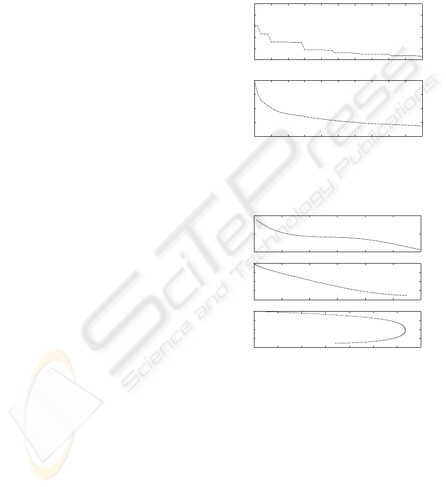
The evolution of the solution over 50 generations
is shown in Fig.1. The control sequence γ(i), the op-
timal trajectory and the velocity V
2
(i) are displayed
in Fig.2. The sign of y is reversed for plotting. It
can be seen from the plots that the angle varies at the
beginning and at the end of the motion, but remains
constant in the middle of the maneuver, resulting in
a dive along a straight line along a considerable por-
tion of the trajectory. This finding agrees well with
the results obtained by Bryson (Bryson, 1999) using
a gradient method.
0 5 10 15 20 25 30 35 40 45 50
−2.75
−2.7
−2.65
−2.6
−2.55
−2.5
Best f
0 5 10 15 20 25 30 35 40 45 50
−2.8
−2.7
−2.6
−2.5
−2.4
Generations
Average f
Figure 1: Convergence of the DVDP solution with gravity,
thrust a=0.05 and drag, with no terminal constraint on y
f
.
x(N) is maximized. With final time t
f
= 5.
0 10 20 30 40 50 60
0
0.5
1
i
gama / ( pi/2 )
0 0.5 1 1.5 2 2.5 3
−2
−1.5
−1
−0.5
0
x / L
c
y / L
c
0 0.05 0.1 0.15 0.2 0.25 0.3 0.35
−2
−1.5
−1
−0.5
0
v
2
/ 2 g L
c
y / L
c
Figure 2: The control sequence, the optimal trajectory and
the velocity V
2
(i) for the DVDP problem with gravity,
thrust a=0.05 and drag. No terminal constraint on y
f
. Final
time t
f
= 5. The sign of y is reversed for plotting.
5 NONLINEAR CONTINUOUS
TIME OPTIMAL CONTROL
In this section, a formulation is developed for the non-
linear continuous time optimal control problem sub-
ject to terminal constraints. Consider the continuous
time nonlinear problem described by a system of or-
dinary differential equations with initial conditions
ICINCO 2005 - INTELLIGENT CONTROL SYSTEMS AND OPTIMIZATION
50

dx/dt = f [x(t), u(t), t] (5.1)
x(0) = x
0
(5.2)
where x ∈ R
n
is the vector of state variables,
u ∈ R
p
, p < n is the vector of control variables and
t ∈ [0, t
f
] is the continuous time. The function f is a
nonlinear function of the state vector, the control vec-
tor and the time t, i.e., f : R
n
x R
p
x R 7→ R
n
.
Next, define a performance index
J[x(t), u(t), t
f
] = φ[x(t
f
)] +
tf
∫
0
L[x(t), u(t), t]dt
(5.3)
φ : R
n
7→ R, L : R
n
xR
p
xR 7→ R
Here L is the Lagrangian function and φ[x(t
f
)] is
a function of the terminal value of the state vector
x(t
f
). In some problems, additional terminal con-
straints can be prescribed through the use of functions
ψ of the state variables x(t
f
)
ψ[x(t
f
)] = 0, ψ : R
n
7→ R
k
, k ≤ n (5.4)
The formulation of the optimal control problem ac-
cording to Bolza consists of finding the control u(t)
such as to maximize the performance index defined
by (5.3), subject to the state equations (5.1) with ini-
tial conditions (5.2) and terminal constraints (5.4). In
the alternative formulation, due to Mayer, the state
vector x
j
, j ∈[1, n] is augmented by an additional
state variable x
n+1
which satisfies the following ini-
tial value problem:
dx
n+1
/dt = L[x(t), u(t), t] (5.5)
x
n+1
(0) = 0 (5.6)
The performance index can then be written as
J(t
f
) = φ[x(t
f
)] + x
n+1
(t
f
) ≡ φ
a
[x
a
(t
f
)] (5.7)
where x
a
= [x x
n+1
]
T
is the augmented state
vector and φ
a
the augmented performance index. We
next define an augmented performance index with ad-
joint constraints ψ and adjoint dynamical constraints
f [x(t), u(t), t ]−dx/dt = 0, with static and dynam-
ical Lagrange multipliers ν and λ as:
J
a
(t
f
) = φ[x(t
f
)]+ν
T
ψ[x(t
f
)]+λ
T
(0)[x
0
−x(0)]
+
tf
∫
0
λ
T
(t)[f[x(t), u(t), t] − dx/dt]dt (5.8)
Introducing a Hamiltonian function
H(t) = λ
T
(t)f[x(t), u(t), t] (5.9)
and rewriting the augmented performance index in
terms of the Hamiltonian, we get
J
a
(t
f
) = φ + ν
T
ψ − λ
T
(t
f
)x(t
f
) + λ
T
(0)x
0
+
+
tf
∫
0
[H(t) − λ
T
(t)x(t)]dt (5.10)
A first order necessary condition for J
a
to reach
a stationary solution is given by the Euler-Lagrange
equations
dλ
T
/dt = −H
x
(t) = −λ
T
(t)f
x
[x(t), u(t), t]
(5.11)
with final conditions
λ
T
(t
f
) = φ
x
[x(t
f
)] + ν
T
ψ
x
[x(t
f
)] (5.12)
The control u(t) satisfies the optimality condition:
H
u
(t) = λ
T
(t)f
u
[x(t), u(t), t] = 0 (5.13)
If we define an augmented function Φ[x(t
f
)] as
Φ[x(t
f
)] = φ[x(t
f
)] + ν
T
ψ[x(t
f
)] (5.14)
then the final conditions can be written in terms
of the augmented function Φ in a similar way to the
problem without terminal constraints
λ
T
(t
f
) = Φ
x
[x(t
f
)] = φ
x
[x(t
f
)] + ν
T
ψ
x
[x(t
f
)]
(5.15)
In the indirect approach to optimal control, the nec-
essary conditions are used to obtain an optimal solu-
tion: the state equations (5.1) with initial conditions
(5.2) have to be solved together with the adjoint equa-
tions (5.11) and the final conditions (5.15). The con-
trol history u(t) is determined from the optimality
condition (5.13). Consequently, this approach leads
to a coupled system of nonlinear ordinary differential
equations with the boundary conditions for the state
variables specified at the initial time t = 0 and the
boundary conditions for the adjoint variables speci-
fied at the final time t = t
f
. This is a nonlinear two-
point boundary value problem (TPBVP) in ordinary
differential equations. Except for some special sim-
plified cases, it is usually very difficult to obtain solu-
tions for such nonlinear TPBVPs analytically. Many
numerical methods have been developed in order to
obtain approximate solutions to this problem.
EVOLUTIONARY COMPUTATION FOR DISCRETE AND CONTINUOUS TIME OPTIMAL CONTROL PROBLEMS
51

6 GODDARD’S OPTIMAL
CONTROL PROBLEM IN
ROCKET DYNAMICS
We now illustrate the above approach with a contin-
uous time optimal control example. We apply the
optimal control formulation described in the previous
section for continuous time dynamical systems to the
study of the vertical climb of a single stage sound-
ing rocket launched vertically from the ground. This
is known in the literature as the Goddard’s problem.
The problem is to control the thrust of the rocket such
as to maximize the final velocity or the final altitude.
There are two versions to this problem: in the first
version, the final mass of the rocket is prescribed and
the final time is free. In the second version, the fi-
nal time is prescribed and the final mass is free. The
second version of this problem will be presented.
Let h(t) denote the altitude of the rocket as mea-
sured from sea level and v(t) and m(t) the velocity
and the mass of the rocket, respectively. Here the
time t is continuous. The trajectory of the rocket is a
vertical straight line. The forces acting on the rocket
are the thrust T (t), which is used as the control vari-
able or control history, the aerodynamic drag force
D(h, v), which is a function of altitude and speed
and the weight of the rocket m(t)g, where m(t) is
the mass and g is the acceleration of gravity, assumed
constant. The equations of motion are:
dh/dt = v (6.1)
mdv/dt = T − D − mg (6.2)
dm/dt = −T/c (6.3)
where the drag force is given by
D(h, v) = D
0
v
2
exp(−h/h
r
) (6.4)
Hereh
r
= 23800 ft is a characteristic altitude and
D
0
is a characteristic drag force given by
D
0
= 0.711T
M
/c
2
(6.5)
where T
M
is the maximum thrust developed by
the rocket. The speed c is the propellant jet exhaust
speed. An important parameter in rocket dynamics is
the thrust to weight ratio τ = T
M
/(m
0
g), where m
0
is the initial mass of the vehicle and g = 32.2 ft/s
2
.
In this example, a ratio of 2 is chosen:
τ = T
M
/(m
0
g) = 2 (6.6)
Here we take a value of m
0
= 3 slugs for a small
experimental rocket. A typical value of the exhaust
speed c and the specific impulse I
sp
for an early
rocket such as the one tested by Goddard is given by
c = (3.264gh
r
)
1/2
= 1581ft/s
I
sp
= c/g = 49.14sec (6.7)
The initial conditions are
h(0) = 0, v(0) = 0, m(0) = m
0
= 3 slugs
(6.8)
The optimal control problem is to find the control
history T (t) such as to maximize the final altitude (or
the altitude at burnout) h(t
f
) in a given time t
f
, where
a value t
f
= 18 sec was used in this example. The
state equations (6.1-6.3) with the initial conditions
(6.8) are to be solved in the optimization process. Be-
fore solving this problem, we first restate the problem
in non-dimensional form. Choosing the characteristic
speed (gh
r
)
1/2
= 875 ft/s and the characteristic time
(h
r
/g)
1/2
= 27.2 sec, we introduce nondimensional
variables, denoted here by primes:
h = h
r
h′, v = (gh
r
)
1/2
v′, t = (h
r
/g)
1/2
t′
m = m
0
m′, T = T
M
T ′, D = T
M
D′ (6.9)
Introducing the variables from Eq.(6.9) in the state
equations (6.1-6.3) and simplifying, the following
system of non-dimensional equations is obtained:
dh/dt = v (6.10)
mdv/dt = τ T − τσ
2
v
2
exp(−h) − m (6.11)
dm/dt = −1.186 στ T (6.12)
In this system of equations (6.10-6.12) all the vari-
ables are non-dimensional and the prime notation has
been omitted. Two independent non-dimensional pa-
rameters characterizing this problem are obtained: the
thrust to weight ratio τ, introduced before and a ratio
of two speeds σ defined by
τ = T
M
/(m
0
g) = 2, T
M
= 193 lbs
σ = (0.711gh
r
)
1/2
/c = 0.467 (6.13)
The non-dimensional initial conditions are:
h(0) = 0, v(0) = 0, m(0) = 1 (6.14)
The optimal control problem is to find the control
history T (t) such as to maximize the final altitude (the
altitude at burnout) h(t
f
) in a given normalized time
ICINCO 2005 - INTELLIGENT CONTROL SYSTEMS AND OPTIMIZATION
52
t′
f
= t
f
/(h
r
/g)
1/2
= 0.662
subject to the state equations (6.10-6.12) and the
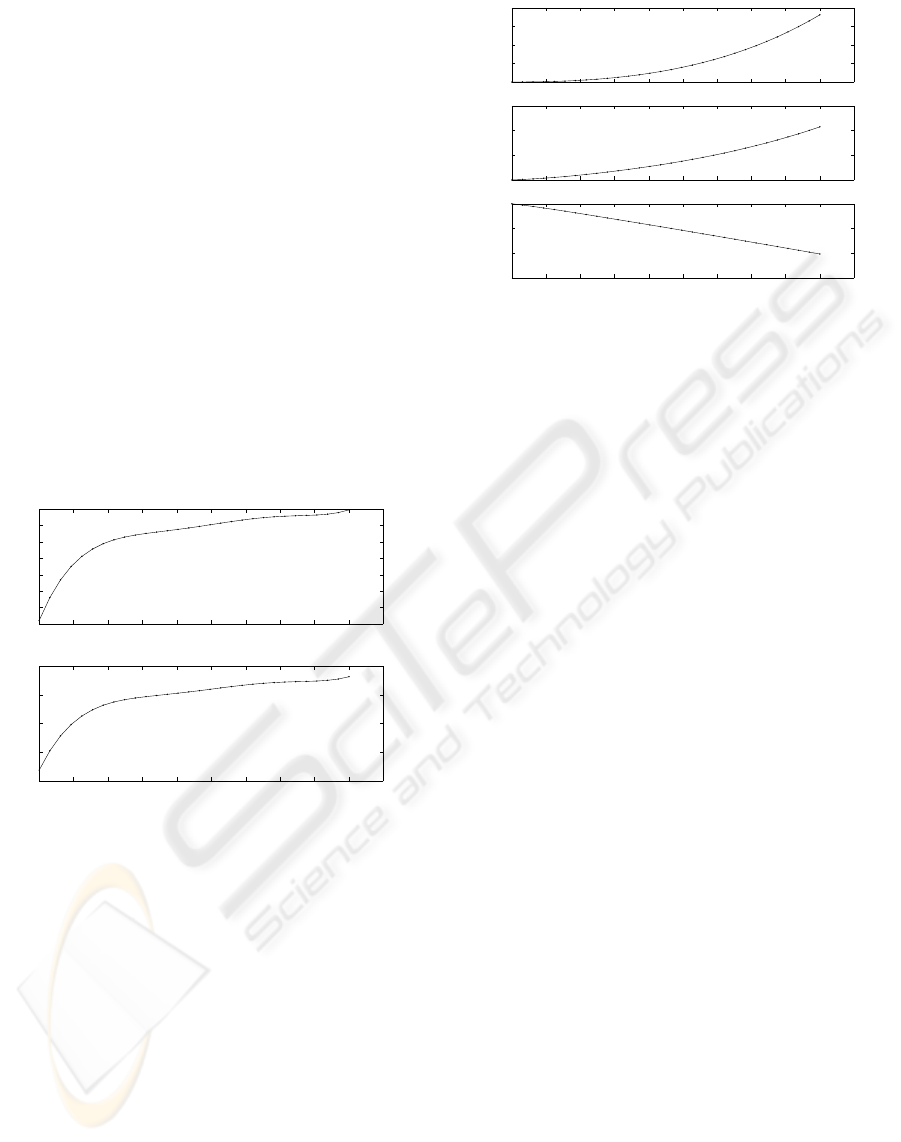
initial conditions (6.14). The results of this contin-
uous time optimal control problem are given in Fig-
ures (3-4). Figure 3 shows the control history of the
thrust as a function of the time in seconds. In the
genetic search, the search range for the normalized
thrust was between a lower bound of (T/T
max
)
L
= 0.1
and an upper bound (T/T
max
)
U
= 1. It can be seen that
the thrust increases sharply during the first two sec-
onds of the flight and remains closer to 1 afterwards.
Figure 4 displays the state variables, the altitude, the
velocity and the mass of the rocket as a function of
time. The mass of the rocket decreases almost linearly
during the flight due to the optimal control which re-
quires an almost constant thrust. This is in agreement
with the results of Betts (J. Betts and Huffman, 1993)
and (A.S. Bondarenko and More, 1999) who used a
nonlinear programming method. See also (Dolan and
More, 2000).
0 2 4 6 8 10 12 14 16 18 20
0.65
0.7
0.75
0.8
0.85
0.9
0.95
1
T/Tmax
0 2 4 6 8 10 12 14 16 18 20
120
140
160
180
200
Thrust (lbs)
time (sec)
Figure 3: The thrust control history. The upper graph dis-
plays the value of the thrust normalized by maximum thrust.
The lower graph shows the actual thrust in lbs.
7 CONCLUSIONS
A new method for solving both discrete time and con-
tinuous time nonlinear optimal control problems with
terminal constraints has been presented. Unlike other
methods that use the first-order necessary conditions
to find the optimum, the present method seeks the best
control history directly by a modified genetic search.
As a consequence of this direct search approach, there
is no need to develop a Hamiltonian formulation and
therefore there is no need to solve a difficult two-point
boundary value problem for the state and adjoint vari-
ables. This has a significant advantage in more ad-
0 2 4 6 8 10 12 14 16 18 20
0
2000
4000
6000
8000
h (ft)
0 2 4 6 8 10 12 14 16 18 20
0
500
1000
1500
v (ft/sec)
0 2 4 6 8 10 12 14 16 18 20
0
1
2
3
time (sec)
m (slugs)
Figure 4: The state variables, the altitude, velocity and mass
of the rocket as a function of time
vanced and higher order problems where it is diffi-
cult to solve the two point boundary value problem
(TPBVP) with large systems of ordinary differential
equations. There is a computational price to be paid,
however, since the method involves repetitive solu-
tions of the initial value problem (IVP) for the state
variables during the evolutionary process.
The method was demonstrated by solving a
discrete-time optimal control problem, namely, the
discrete velocity direction programming problem
(DVDP) of a body with the effects of gravity, thrust
and hydrodynamic drag. Benchmark problems of this
kind were pioneered by Bryson who used analytical
and gradient methods. This discrete time problem was
solved easily using the proposed approach and the re-
sults compared favorably with the results of Bryson.
The method was also applied to a continuous time
nonlinear optimal control problem, the Goddard’s
problem of rocket dynamics. The results compared
favorably with published results obtained by a non-
linear programming method.
REFERENCES
A.S. Bondarenko, D. B. and More, J. (1999). Cops: Large
scale nonlinearly constrained optimization problems.
In Argonne National Laboratory Technical Report
ANL/MCS-TM-237.
Betts, J. (2001). Practical Methods for Optimal Control Us-
ing Nonlinear Programming. SIAM, Society for In-
dustrial and Applied Mathematics, Philadelphia, PA.
Bryson, A. (1999). Dynamic Optimization. Addison-
Wesley Longman, Menlo Park, CA.
Coleman, T. and Liao, A. (1995). An efficient trust region
method for unconstrained discrete-time optimal con-
trol problems. In Computational Optimization and
Applications, 4:47-66.
EVOLUTIONARY COMPUTATION FOR DISCRETE AND CONTINUOUS TIME OPTIMAL CONTROL PROBLEMS
53

Dolan, E. and More, J. (2000). Benchmarking optimization
software with cops. In Argonne National Labo-ratory
Technical Report ANL/MCS-TM-246.
Dunn, J. and Bertsekas, D. (1989). Efficient dynamic pro-
gramming implementations of newton’s method for
unconstrained optimal control problems. In J. of Op-
timization Theory and Applications,63, pp. 23-38.
Fogel, D. (1998). Evolutionary Computation, The Fossil
Record. IEEE Press, New York.
Fox, C. (1950). An Introduction to the Calculus of Varia-
tions. Oxford University Press, London.
J. Betts, S. E. and Huffman, W. (1993). Sparse nonlin-
ear programming test problems. In Technical Report
BCSTECH-93-047. Boeing Computer Services, Seat-
tle, Washington.
Jacobson, D. and Mayne, D. (1970). Differential Dynamic
Programming. Elsevier Science Publishers, Amster-
dam, Netherland.
Kirkpatrick, G. and Vecchi (1983). Optimization by simu-
lated annealing. In Science, 220: 671-680. AAAS.
Laarhoven, P. and Aarts, E. (1989). Simulated Annealing:
Theory and Applications. Kluwer, Amsterdam.
Liao, L. and Shoemaker, C. (1991). Convergence in uncon-
strained discrete-time differential dynamic program-
ming. In IEEE Transactions on Automatic Control,
36, pp. 692-706. IEEE.
L.S. Pontryagin, V.G. Boltyanskii, R. G. and Mishchenko,
E. (1962). The Mathematical Theory of Opti-
mal Processes. translated by K.N. Trirogoff, L.W.
Neustadt (Ed.), Moscow, interscience, new york edi-
tion.
Mayne, D. (1966). A second-order gradient method for
determining optimal trajectories of nonlinear discrete
time systems. In International Journal of Control, 3,
pp. 85-95.
Michalewicz, Z. (1992). Genetic Algorithms + Data Struc-
tures= Evolution Programs. Springer-Verlag, Berlin.
Murray, D. and Yakowitz, S. (1984). Differential dynamic
programming and newton’s method for discrete opti-
mal control problems. In J. of Optimization Theory
and Applications, 43:395-414.
Ohno, K. (1978). A new approach of differential dynamic
programming for discrete time systems. In IEEE
Transactions on Automatic Control, 23, pp. 37-47.
IEEE.
Pantoja, J. (1988). Differential dynamic programming and
newton’s method. In International Journal of Control,
53: 1539-1553.
Schwefel, H. (1995). Evolution and Optimum Seeking. Wi-
ley, New York.
Yakowitz, S. and Rutherford, B. (1984). Computational as-
pects of discrete-time optimal control. In Appl. Math.
Comput., 15, pp. 29-45.
Z. Michalewicz, C. J. and Krawczyk, J. (1992). A mod-
ified genetic algorithm for optimal control problems.
In Computers Math. Appl., 23(12),8394.
ICINCO 2005 - INTELLIGENT CONTROL SYSTEMS AND OPTIMIZATION
54
