
ANN-BASED MULTIPLE DIMENSION PREDICTOR FOR
SHIP ROUTE PREDICTION
Tianhao Tang, Tianzhen Wang
Institute of Electrical & Control Engineering,Shanghai Maritime University, 1550 Pudong Road,Shanghai,China
Keywords: Nonlinear time series model, adaptive predictor, artificial neural networks, data mining.
Abstract: This paper presents a new multiple dimension predictive model based on the diagonal recurrent neural
networks (PDRNN) with a combined learning algorithm. This method can be used to predict not only
values, but also some points in the multi-dimension space. And also its applications in data mining will be
discussed in the paper. Some analysis results show the significant improvement to ship route prediction
using the PDRNN model in database of geographic information system (GIS).
1 INTRODUCTION
The problem of prediction is denoted to estimate the
output of future according to input and output of
now and past in some system. Since Kolmogorov
presented a linear optimal predictor in 1941,
different kinds of trend analysis methods and
prediction models have been used for forecasting
and control. In this field, the time series prediction
model (Box and Jenkins, 1970) and the self-tuning
predictor (Wittenmark, 1974) were two kinds of
classical prediction methods. The tradition
prediction theories based on time series were
developed from linear auto recurrent moving
average (ARMA) models. And then these theories
were extended to nonlinear process. But, if using the
tradition predictive theories, it needs to solve the
problems: system modelling, parameter estimating,
model modifying and trend forecasting on-line.
In order to solve these problems, some
intelligent prediction methods were discussed, in
which the forward neural networks with BP
algorithm were used more popularly. Prediction
based on ANN has made an overwhelming impact
on many disciplines. But there are some difficulties
in prediction, particularly in the prediction of multi-
variable and non-steady dynamic process.
Recent years, scholars had done much research,
and made some progresses in this filed. We have
researched predictive models using neural networks,
such as an ANN-based nonlinear time series model
for fault detection and prediction in marine system
(Tang, 1998) and an adaptive predictor based on a
recurrent neural network for fault prediction and
incipient diagnosis (Tang, 2000). Furthermore a
direct multi-step adaptive predictor based on a
diagonal recurrent neuron network was presented for
intelligent system monitoring (Dou, 2001). These
models increased the precision and self-adaptation
of prediction in a manner.
However, there existed a problem: former
prediction methods based on time series models
could only approach or predict processes with one
kind of attribute, such as temperature, pressure and
flow in an industry process, or stock values and
GDP in the economic process. In this case, every
parameter must be separately denoted if using a
traditional time series model in the dynamic process.
But some objects have more than two kinds of
attributes, and must be represented as one predictive
model. For example, a ship route has two kinds of
attributes: longitude and latitude. A satellite position
has three kinds of attributes: longitude, latitude and
altitude. So the question of how to predict objects
with several attributes is an important problem in
practice.
This paper discusses self-adaptation prediction
methods based on ANN, and presents a multi-
dimension predictive model based on parallel
diagonal recurrent neuron network (PDRNN) with
TD-DBP combined algorithms for time series multi-
step forecasting. The paper takes a step forward to
use this model in data mining of GIS. Some
simulation resolves show the model is able to predict
a ship’s route according to its position from GPS.
2 PRINCIPLE OF ANN-BASED
PREDICTOR
The basic issue of a predictor can be described as:
if the past output value series {x
t
} is known, then
52
Tang T. and Wang T. (2005).
ANN-BASED MULTIPLE DIMENSION PREDICTOR FOR SHIP ROUTE PREDICTION.
In Proceedings of the Second International Conference on Informatics in Control, Automation and Robotics - Signal Processing, Systems Modeling and
Control, pages 52-59
DOI: 10.5220/0001168200520059
Copyright
c
SciTePress
try to design a predictor to obtain the future output
value of forward d-step x
t+d
under the condition
of the minimum predictive errors. If x
t+d
is expressed
as , the model of predictor can be described as
follows:
),,()(
ˆ
1
PtXfdx
tt −
= (1)
Where X
t-1
= [x
1
,
x
2
, …, x
t-1
]
T
is the past output
value vector, i.e. historical data.
f (·) is a certain nonlinear function.
P is the parameter set of the system model.
The predictor is called the minimum covariance
optimal predictor, because the covariance of the
predictive error is used for criterion function J as
follows:
min))(
ˆ
( →−=
+
kxxVarJ
tkt
(2)
2.1 RNN-based One-step Predictor
The ANN-based models could be used to construct
an adaptive optimal predictor for model
identification, parameter correction and value
prediction. Assuming that a class of nonlinear
processing can be represented by a nonlinear
autoregressive moving average (NARMA) model,
the NARMA (p, q) model is written as:
tqtttptttt
eeeexxxgx +=
−−−−−−
),,,,,,,,(
2121
"""
(3)
Where is an unknown smooth function, and it is
assumed that E (e
t
│ x
t-1
, x
t-2
,… ) = 0 and e
t
has a
finite variance Var ( e
t
) = σ
2
. In this case, an
approximated condition mean predictor based on the
finite past of observations is given by
(
)
qtttptttt
eeexxxgx
−−−−−−
=
ˆ
,,
ˆ
,
ˆ
,,,,
ˆ
2121
"" (4)
Where
qtttjxxe
jjj
−−−=−= ,,2,1
ˆˆ
"
For NARMA (p, q) modelling and predicting, a
recurrent neural network was presented (Connor,
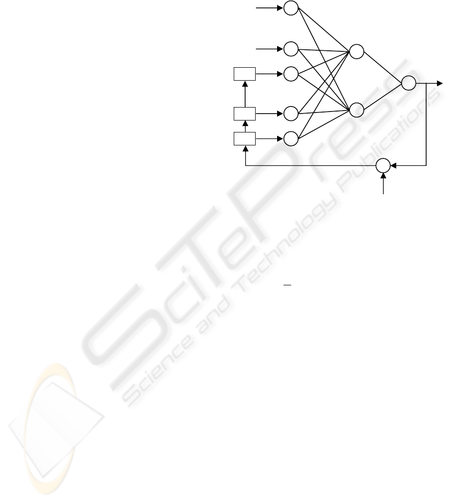
1994). The recurrent network topology is shown in
figure 1. This recurrent neural network (RNN) can
be used to approximate the NARMA (p, q) model.
The output of the basic RNN-based predictor is
f(s)W
o
=
t
x
ˆ
(5)
θeWxWs
ehih
++= (6)
Where f (⋅) is a Sigmoid function vector or other
finite continuous monotonically increasing function
vectors;
s is a state vector of the hidden layer;
W
ih
is the weight matrix between the input
layer and the hidden layer;
W
eh
is the weight matrix from feedback units
to hidden units;
x is the input vector;
e is the error vector;
θ is a threshold vector.
Figure 1: Recurrent network for NARMA models
The parameters of W
o
, W
ih
and W
eh
are
estimated by a dynamic BP learning algorithm
(Williams, 1990). That is by learning of RNN to
minimize the following error function:
∑
+=
−=
N
pt
tt
xxE
1
2
)
ˆ
(
2
1
(7)
But, just one step prediction will make by the
basic predictor. So some improvement RNN-based
predictors had been discussed (Tang, 2000).
2.2 RNN-based Multi-step Predictor
In order to implement the multi-step prediction, the
NARMA model should be extended to:
()
jdttt
eidXgdx
−+
−=
ˆ
,)(
ˆ
)(
ˆ
(8)
Where
q21jjdxxe
tjdtjdt
,,,,)(
ˆˆ
"=−−=
−+−+
[]
T
ptttttt
xxxdxdxidX
−−
−−=− ,,,,),2(
ˆ
),1(
ˆ
)(
ˆ
1
""
The output of the multi-step RNN model is
f(s)Wx
ot
=
ˆ
(9)
Where
θeWxWs
ehih
++=
)(
ˆ
dx
t
)(⋅g
.
.
.
.
.
.
x
t-1
x
t-p
W
i
h
W
eh
W
o
z
-
1
+
-
f
.
.
.
z
-
1
z
-
1
f
e
t-q
e
t-2
e
t-1
e
t
x
t
^
x
t
ANN-BASED MULTIPLE DIMENSION PREDICTOR FOR SHIP ROUTE PREDICTION
53
T
dttt
xxx ]
ˆˆˆ
[
ˆ
1 ++
= "
t
x
And the error function is
∑
+=
−−=
N
pt
E
1
ˆˆ
(
2
1
)x(x)xx
tt
T
tt
(10)
Using the dynamic BP learning algorithm, and
assuming that the dimensions of the input, error,
hidden and output matrices could be represented as i,
e, h, and o, the iteration formulae of the weight
values of the RNN prediction model can be obtained
as following:
() ()
W
WW
∂
∂
η
E
kk −=+ 1
(11)
To the weight values of the output layer, there is
t
oh
o
esfI
W
)(
1
)(
∑
+=
×
−=
N
Pt
E
∂
∂
(12)
Where
ttt
xxe
ˆ
−=
(13)
And I is an identity matrix.
To the weight values between the hidden layer
and input layer, there is
∑
+=
×
⋅
∂
∂
⋅
∂
∂
+⊗⋅−=
∂
∂
n
pt 1
)(
)((
t
T
o
T
eh
ih
(h)h)(i
ih
eW
s
sf
)W
W
e
xII
W
E
(14)
Where ⊗ is Kronecker product.
⎥
⎦
⎤
⎢
⎣
⎡
∂
∂
∂
∂
∂
∂
=
∂
∂
−
−−
ihihihih
WWWW
e
qt
tt
e
ee
,,,
21
" (15)
To the weight values of the hidden layer and
feedback units, there is
()
()
t
T
N
pt
T
t
E
eW
s
sf
W
W
e
eII
W
eh
eh
hhe
0
1
eh
∑
+=
×
∂
∂
⎟
⎟
⎠
⎞
⎜
⎜
⎝
⎛
∂
∂
+⊗−=
∂
∂
(16)
Where
⎥
⎦
⎤
⎢
⎣
⎡
∂
∂
∂
∂
∂
∂
=
∂
∂
−
−−
eheheheh
WWWW
e
qt
tt
e
ee
,,,
21
" (17)
3 DRNN PREDICTIVE MODELS
In order to obtain the optimal predictive value of the
future output of the analyzed system based on its
historical data, a stochastic dynamic model of the
analyzed system should be set up, which can modify
the model parameter adaptively. A diagonal
recurrent neural network was used to represent the
dynamic process based on NARMA model (Dou,
2001). The NARMA model is defined as:
)
ˆ
,,
ˆ
,,,,(
ˆ
11121
eexxxhx
tttdt
""
−−−+
= (18)
Where
jjj
xxe
ˆˆ
−= , j = t-1, t-2, …, 1;
h(·) is a nonlinear function.
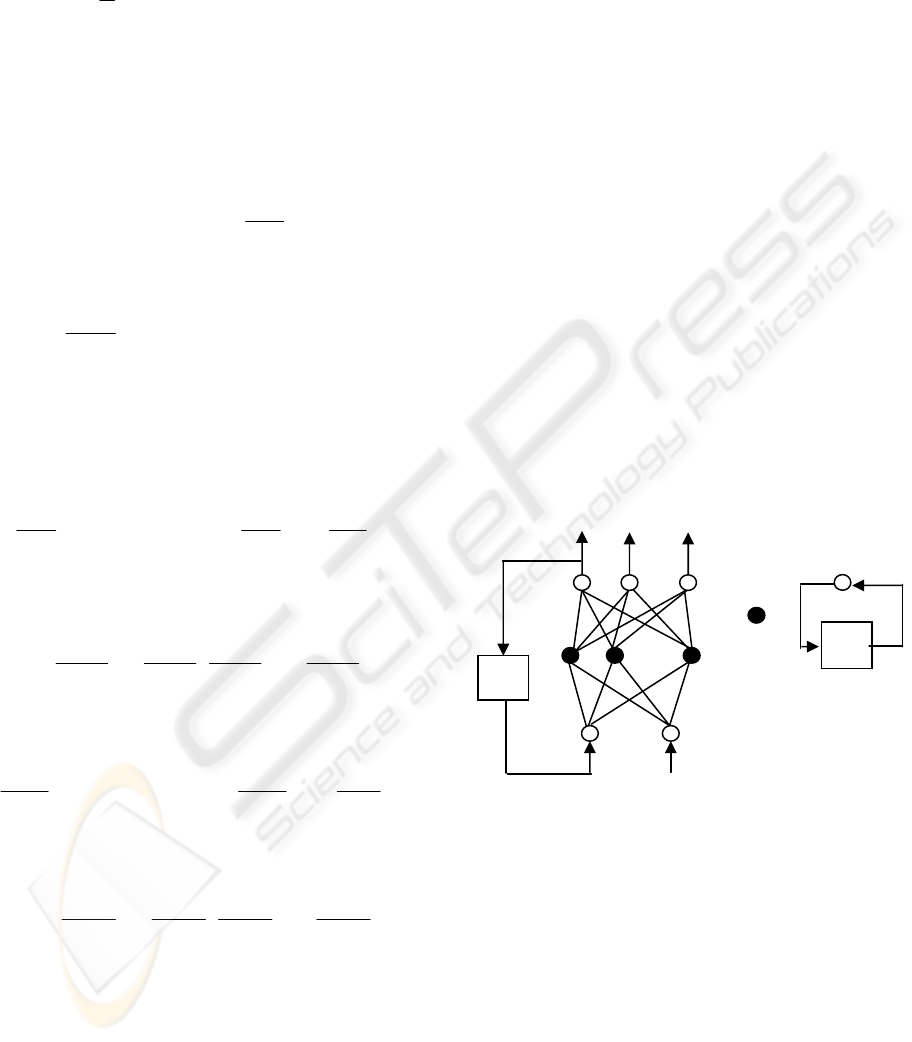
Figure 2 shows the structure of the DRNN-based
predictive model. The neural network model with
two inputs and several outputs includes three layers.
In order to realize direct multi-steps prediction, the
output layer composes of d linear neural units. And
the middle layer (i.e. hidden layer) makes up NH
nonlinear dynamic neurons whose map function is
the sigmoid function, and each of the hidden unit
includes a self-feedback with one step delay
(recursion layer). The input layer includes two linear
neurons, and one of them accepts x
t-1
as input signal,
another accepts , which is one-step delay of the
output x
t
. This network can be regarded as a
parsimonious version of the Elman-type network. It
has a diagonal structure, that is, there is no
interaction between different dynamic neurons.
x
t
x
t +1
x
t+d
…
=
A
j
W
ij
…
a
1j
a
2j
Figure 2: DRNN-based predictive model
The transfer function of this network is described
as follows. Suppose w
ij
(i =1, 2, …, NH; j =1, 2, …,
d) are the connection weights of the output layer, A
i
(i=1, 2,…, NH) are the connection weights of the
recursion layer, a
1i
(i =1, 2, … , NH) are the
connection weights of the input x
t-1
to each of the
hidden units, a
2i
(i = 1, 2, …, NH) are the connection
weights of the input to each of the hidden units,
the output of the neural unit of the output layer is
expressed as , (j =1, 2,…d), the output of an
neurons of hidden layer is expressed as H
i
( t ), ( i
=1, 2,…, NH), the input of the neural unit of the
hidden layer is expressed as V
i
( t ) (i = 1, 2, …,
1
ˆ
−t
x
1−t
x
z
-
1
z
-
1
1
ˆ
−t
x
)(
ˆ
jx
t
)(
ˆ
jx
t
ICINCO 2005 - SIGNAL PROCESSING, SYSTEMS MODELING AND CONTROL
54

NH), then the map relations of the DRNN are shown
as fellows:
])([)(
ˆ
NH
1
oj
i
iijt
tHwjx
θ
−=
∑
=
(19)
Where
))(()(
hiiNi
tVgtH
θ
−= (20)
)
ˆ
()()1()(
212111
θ
θ
−+−+−=
−− titiiii
xaxatHAtV (21)
is sigmoid function,
θ
oj
is the threshold of
the neural unit of output layer,
θ
hi
is the threshold
of the neuron of hidden layer. The initial conditions
of this model are H
i
(0) = 0 and V
i
(0) = 0. So the
transfer function of the neural network is a nonlinear
continuous function, and the output of the neural
network is an appropriate nonlinear function of
all input signals (x
1
, x
2
, …, x
t-1
).
It is known that the supervised learning
algorithm based on the error between the actual
output and the anticipant output is not suitable for
the direct multi-step predictive model. And a neural
network with the fixed structure and parameters is
difficult or even impossible to express the inherent
dynamic performance of the uncertain nonlinear
systems. For this reason the temporal difference
(TD) learning algorithm and the dynamic back-
propagation (DBP) algorithm are synthesized for the
network training. The combined learning algorithm
will adaptively modify the parameters of the
predictive model according to the errors between the
predictive value and the actual detective value.
Suppose P
t
j
is the output of the jth output
neuron at t time, i.e. , P
t+1
j-1
is the output of
the (j-1)th output neuron at t+1 time, i.e. . It
is obvious that P
t
j
and P
t+1
j-1
are the predictive
output value of the analyzed system at the same
time. And they should be equal if the prediction is
accurate. So the P
t+1
j-1
can be used as the
expectant output of the P
t
j
. This is the basis of
TD learning algorithm. The training error of one
learning sample of the DRNN is expressed as:
∑
=
+
−=
K
j
tjt
jxxe
0
2
))(
ˆ
(
2
1
(22)
According to TD learning algorithm, it can be
expressed as
∑
=
+
−=
K
j
t
t
j
jxPe
0
21
))(
ˆ
(
2
1
(23)
Here P
0
t+1
is defined as the expectant output of x
t
at t time.
4 A MULTI-DIMENSION
PREDICTOR BASED ON
PDRNN
One dimension predictive model can predict an
object with one kind of attribute. A multi-dimension
predictive model can predict an object with more
than one kind of attribute at the same time. In the
multi-dimension predictive model, there are
different relations in different attributes and the
relations can be changed by a dynamic process. For
this reason, ANN-based adaptive predictors must be
introduced to modify the parameters of a predictive
model on-line.
4.1 The Framework of PDRNN
Model
In order to solve the predictive problem of objects
with multi-attributes, this paper presents a new
multi-dimensional predictive model based on
the
diagonal recurrent neural networks (PDRNN) with a
parallel combined learning algorithm. Fig. 3 shows
the framework of PDRNN model. There are four
layers in this model, the first layer is the network
input layer; the second layer is the network input
assignment layer; the third layer is the network
hidden layer, in which every hidden unit includes a
self-feedback with one step delayed; the forth layer
is the network output layer, (the network output
layer connects with the network input layer through
one-step feedback). There are n dimension variables
to input paralleled in the network input layer. It
solves the problem that only one variable can be
input in some one dimension predictive models, and
the PDRNN model can predicts an object with
multiple variables and attributes.
4.2 The Mathematical Description of
the PDRNN Model
As shown in figure 3, there are p input units in the
network input layer, every input unit has n
dimension variables, can be obtained by with
one step delayed, so each attribute variable has p-1
input values in this network every time in fact. The
network input assignment layer assigns n values of
each variable to n sub-input layers paralleled, as
shown in equation (24). The hidden layer has n sub-
hidden layers paralleled, every sub-hidden layer has
)(
ˆ
jx
t
)(
ˆ
jx
t
)(
ˆ
jx
t
t
X
1+t
Z
)(⋅
N
g
ANN-BASED MULTIPLE DIMENSION PREDICTOR FOR SHIP ROUTE PREDICTION
55
NH
1
(the number of sub hidden layer) nonlinearity
units with S functions or T functions, the value of
NH
1
can be changed, and every sub-hidden layer has
self-feedback with one step delayed. In this network,
n paralleled sub-networks consisted of the sub-input
layers and sub-hidden layers, all the parallel sub-
networks respectively train different attributes at the
same time. This network neglected the relations in
the different attributes and attribute values. There
are k linear units in the network output layer, which
can do d-step prediction at most. The mathematical
model could be described as follows:
The network input layer
],,,[
1 pttt
XXX
−−
"
Where
[
]
n
tttt
XXXX ,,,
21
"= (24)
The Ith parallel sub-network’s sub input layers:
[
]
I
pt
I
t
I
t
XXX
−−
,,,
1
" (25)
The I th parallel sub-network’s sub hidden
layers:
))(()( tVgtH
i
I
N
i
I
=
(26)
In equation (26), at every t time, is the
output of the ith hidden unit in the Ith parallel sub-
network, is Sigmoid (S) function or Tangent
(T) function. And there:
∑
=
−
+−=
I
i
t
I
i
I
i
I
i
I
i
I
XwtHAtV
N
1
1
)1()( (27)
In equation (27), at every t time, is the sum
of all the inputs in the ith hidden layer of the I th
parallel sub-network, is the normalized (relative)
fulfilment weights between the sub-input layer and
sub-hidden layer of the I th parallel sub-network,
is the self-recurrent layer’s relative weights of the ith
hidden unit in the I th parallel sub-network. is
defined as the output of the j th output unit and
includes all the attribute values at this time. So the
output variables of the network model could be
written by equation (28) as below:
⎜
⎜
⎝
⎛
=
∑∑
==
+
12
NH
1
NH
1
2211
),(),(
ii
iijiij
jt
tHatHaZ
⎟
⎟
⎠
⎞
∑
=
n
i
i
n
ij
n
tHa
NH
1
)(," (28)
Where
∑
=
+
=
I
i
I
i
I
ij
I
jt
tHaZ
NH
1
)(
is the jth output layer’s output of the I th attribute at
t time. In the initialization, the threshold value of all
the nerve units were neglected at every t time, and
0)0( =
i
I
H
)(tH
i
I
)(⋅
N
g
I
W
I
i
A
jt
Z
+
)(tV
i
I
Figure 3: Multi-dimension predictive model based on PDRNN
…
…
…
…
…
…
…
…
1+t
Z
2+t
Z
kt
Z
+
t
X
1−t
X
pt
X
−
t
X
2
t
X
1
t
X
3
1
2
−t
X
1
1
−t
X
1
3
−t
X
pt
X
−
2
pt
X
−
1
pt
X
−
3
1−
z
ICINCO 2005 - SIGNAL PROCESSING, SYSTEMS MODELING AND CONTROL
56

5 THE LEARNING ALGORITHM
This paper combines the time different method (TD)
and dynamic BP method to train PDRNN model. If
as the
jth output of the Ith attribute at t time,
is the predictive value of the
Ith attribute at t+j time,
is real value of the
Ith attribute at t+j time in
the future.
In the ideal condition, is equal to ,
but usually there are some errors in practice. It could
be represented by following error function.
()
2
0
2
1
∑
=
+
+
−=
kN
j
I
jt
jt
II
I
ZXe (29
)
Equation (29) is the training error of the
Ith
attribute at
t+j time. Here use a dynamic BP method
to correct relative weighs. The learning algorithm is
as follows
()
)(tHXZ
a
X
X
e
a
e
i
I
jt
I
jt
I
I
ij
it
I
it
I
I
I
ij
I
++
+
+
−−=
∂
∂
∂
∂
=
∂
∂
(30)
Where are the normalized (relative) fulfilment
weights between the sub hidden layer and sub output
layer of the Ith paralleled sub-network.
The formula corrected of as follows:
)()()(
)()1(
tHZXta
a
e
tata
I
i
I
jt
I
jt
II
ij
I
ij
I
II
ij
I
ij
++
−+=
∂
∂
−=+
ξ
ξ
(31)
Where is learning parameter of the Ith attribute’s
output layer, is the normalized (relative)
fulfilment weights between the sub input layer and
sub hidden layer of the Ith paralleled sub-network.
∑
∑
=
++
+
=
+
∂
∂
−−=
∂
∂
∂
∂
∂
∂
−=
∂
∂
kN
j
I
ij
I
i
I
ij
I
jt
I
jt
ij
I
i
I
i
I
it
I
kN
j
it
I
I
ij
I
I
I
I
w
H
wZX
w
tH
tH
X
X
e
w
e
0
0
)(
)(
)(
(32)
The formula is corrected for as follows:
)()()(
)()1(
0
tQaZXtw
w
e
twtw
I
ij
I
ij
kN
j
I
jt
I
jt
II
ij
I
ij
I
II
ij
I
ij
I
∑
=
++
−+=
∂
∂
−=+
η
η
(33)
Where is learning parameter of the Ith attribute’s
input layer;
are the self-recurrent layer’s relative weights.
)()(
)(
)(
0
0
tPaZX
A
tH
tH
X
X
e
A
e
I
i
I
ij
kN
j
I
jt
I
jt
i
I
i
I
i
I
it
I
kN
j
it
I
I
i
I
I
I
I
∑
∑
=
++
+
=
+
−−=
∂
∂
∂
∂
∂
∂
−=
∂
∂
(34)
Where
I
i
I
I
i
A
e
P
∂
∂
=
, and 0)0( =
I
i
P .
The formula corrected of
I
i
A as follows:
I
i
I
ij
kN
j
I
jt
I
jt
II
i
I
i
I
II
i
I
i
PaZXtA
A
e
tAtA
I
∑
=
++
−+=
∂
∂
−=+
0
)()(
)()1(
µ
µ
(35)
Where is the learning parameter of the Ith
attribute’s self-recurrent layer.
First is to adjust the network framework, make
sure of the number of input layers, hidden layers and
output layers, and the number of maximal learning
steps. The above parameters are significant for
predictive accuracy. Second initialize the network
(for new data, the initialization is random), then
ANN begins learning. Equation (29) serves as a
standard to judge the predictive value of each
attribute. In order to avoid the learning of ANN
falling into a dead area, the learning step could be
adjusted according to different attribute values. Here
a “
e
” function was presented, equation (36) serves
as a standard to judge the predictive values of all the
attributes.
∑
=
−
=
n
kt
t
E
kn
e
1
(36)
And
∑
=
=
m
I
I
tt
eE
1
2
)( (37)
Where is the error between the real value and the
predictive value of the Ith attribute at t time, can
be changed according to different attributes.
e
is
the average error, used to judge the convergence of
the multi-dimension predictive model based on
PDRNN. Because the initialization of ANN is
random, the first couple of predictive values may be
not very good,
e
is computed from the kth
predictive value. The training will be stopped when
jt
I
Z
+
jt
I
X
+
jt
I
Z
+ jt
I
X
+
ij
I
a
ij
I
a
I
ξ
ij
I
w
ij
I
w
I
η
I
i
A
I
µ
I
t
e
t
E
ANN-BASED MULTIPLE DIMENSION PREDICTOR FOR SHIP ROUTE PREDICTION
57
e
is up to standard, or reset up the network
framework until
e
confirms to requirements.
6 SIMULATIONS AND
APPLICATION
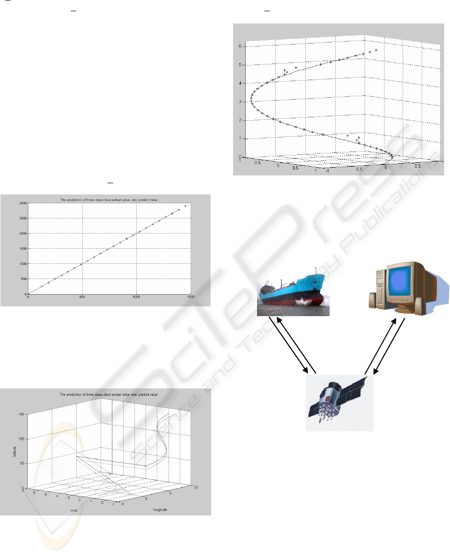
The prediction based on PDRNN extends ANN-
based time series prediction model from a single
attribute to a multi-attribute. Figure 4 is a three-step
predictive value contrasting with real values of
straight line, real lines are real values, “*” indicates
the predictive values. The points of straight line have
two kinds of attributes, every parallel sub-network
has ten sub input layers and fifteen sub hidden
layers. T function is used in the hidden units, the
maximum of e is 2.265e
-5
,
e
is 8.36e
-8
.
Figure 5 is a three-step predictive value of
nonlinearity as follows:
⎭
⎬
⎫
⎩
⎨
⎧
<≤
<≤×
=
ππ
π
42,)(
20,2
xxSin
xx
y
Figure 6 is a three-step predictive value of 3D curve
contrasting with real value, T function is used in the
hidden units, every parallel sub-network only has ten
sub input layers and fifteen sub hidden layers. The
learning step of 3D curve is more than 2D curve.
The maximum predictive error of 3D curve is
0.0011,
e
is 8.265e
-4
.
An application process for GIS in Marine
Engineering with the predictor based on PDRNN is
shown in figure 7.
In the system, data recorded abundant ship
positions from GPS, and established a database
through ACCESS. The software of GIS is ArcView
3.2 of ESRI (Goodchild, 1992). ArcView 3.2 called
the data from ACCESS, and eliminated unnecessary
data by applying ArcView 3.2. After data pre-
processing, the ship route could be selected and
drawn in an electronic chart. Using the PDRNN
predictor the tracking of the ship route could be
forecasted.
The process of ship route prediction by means of
a PDRNN model is as follows: first, get the
distribution data of the ship’s position from GPS
(Wang, 2003), then select sample points. In this
Figure 7: GIS in Marine Engineering
S
teering
Ships
D
isposing
by Com-
puter
P
redicting
Ship
Route
Collecting
Ship'
s
P
osition
GPS
Figure 4: Predictive value contrasting
Figure 5: Prediction of nonlinearity
Figure 6: Prediction of 3D curve
ICINCO 2005 - SIGNAL PROCESSING, SYSTEMS MODELING AND CONTROL
58

paper, the each sample point was selected every 2.5
hours. Figure 8 is a selected ship route. Finally, the
ship route was predicted by means of a PDRNN
model.
Figure 9 is another prediction resolve of a ship
route. This chart shows that this ship route is a
variant random process, but the predictive algorithm
based on a PDRNN model can follow this process,
and do three-step prediction. The predictive
maximum error of the ship route is 1.065e
-14
,
e
is
3.326e
-15
. Thus the error of prediction is small.
7 CONCLUSIONS
As mentioned above, the NARMA models based on
the recurrent neural networks with a dynamic BP
algorithm is suited for trend prediction. This paper
presents a multi-dimension predictive model based
on PDRNN. This predictor could store in memory
all the past input information, network output is
some nonlinear function of all the past input, and
this model can realize a nonlinear dynamic mapping.
As a predictive model, the framework is very
simple, the dynamic behavior of this model could
regulate network frameworks with self-adaptation,
and this model could predict an object with multi-
attribute. Moreover, this paper has presented an “
e
”
function, which can judge if the whole network
structure confirms to requirements, and has
presented an “input plus” method, which can reduce
the training time. The application in ship routing
prediction shows the new predictive model is better
to predict a multiple dimension dynamic process.
REFERENCES
Box, G. E. P. And Jenkins, G. M., 1970. Time series
analysis of forecasting and control
. Holden-day, San
Francisco.
Connor, J. T., Martin R. D. and Atlas L. E., 1994.
Recurrent neural networks and robust time series
prediction. In
IEEE Trans. on neural networks, No.5,
p. 240-254.
Dou, J. and Tang, T., 2001. A DRNN-based direct multi-
step adaptive predictor for intelligent systems. In
Proceedings of the IASTED International Conference
on Modelling, Identification, and Control
, vol.2,
p.833-838, Innsbruck, Austria.
Goodchild, M. F., 1992. Geographic data modeling. In
Computers and Geosciences, Vol. 18, No. 4, pp.401-
408.
Tang, T.
et al., 1998. ANN-based nonlinear time series
models in fault detection and prediction. In
Preprint of
IFAC Conference on CAMS'98
, p.335-340, Fukuoka,
Japan.
Tang, T. et al., 2000. A RNN-based adaptive predictor for
fault prediction and incipient diagnosis. In
UKACC
Control 2000
, Proceedings of the 2000 UKACC
International Conference on Control
. Cambridge, UK.
Wang, T., Hao, R. and Tang, T., 2003. A data mining
method for GIS in marine engineering. In
Navigation
of China
. No. 3, p.1-4.
Williams, R. j. and Peng, J., 1990. An efficient gradient-
based algorithm for on-line training of recurrent neural
networks. In
Neural Computation, No.4, p.490-501.
Wittenmark, B. A., 1974. A self-tuning predictor.
IEEE
Trans. on Automatic Control
, No.6, p.848-851.
Figure 8: The ship route
in GIS
Figure 9: The prediction of ship route
ANN-BASED MULTIPLE DIMENSION PREDICTOR FOR SHIP ROUTE PREDICTION
59
