A SMOOTHING STRATEGY FOR PRM PATHS

Application to 6-axes MOTOMAN manipulator

Reda Guernane, Mahmoud Belhocine

Divison Robotique et Productique , Centre de Développement des Technologies Avancées,CDTA, Cité 20 août 1956,

P 1

Haouch Oukil, Baba Hassen,Alger, Algeria

Keywords: Probabilistic Roadmap, A*, smoothing, motion planning, 6-axis manipulator, collision checks.

Abstract: This paper describes the use of the probabilistic motion planning technique SBL “Single-Query

Bidirectional Probabilistic Algorithm with Lazy Collision Checking” or in motion planning for robot

manipulators. We present a novel strategy to remedy the PRM “Probabilistic Roadmap” paths which are

both excessively long and velocity discontinuous. The optimization of the path will be done first through

Coarse optimal lazy A* optimization and then through a Fine cutting-triangles-edge one, the edges

discontinuities are smoothed with cubic polynomials taking the robot’s specific Dynamic and Cinematic

constraints. The whole strategy is applied to the 6 axes robot Manipulator MOTOMAN SV3X.

1 INTRODUCTION

The motion planning problem has been in a great

difficulty solving path planning for real industrial

robot manipulator which are usually 6 or above

degrees of freedoms (dofs). The traditional

techniques (Latombe, 1991) can hardly solve

problems until 4 or 5 dofs, while its known to be

definitely impossible for 6 dofs in 3D space.

The introduction of random techniques in

roadmap generation (Kavraki, 1996) has greatly

simplified the planning problem, theirs greatest

advantages being, easiness of understanding,

implementing, they can deals with complicated

scene and can solve problem with high number of

dofs.

Their idea consists of randomly sampling the

configuration space (Lozano-Péréz, 1979) of the

robot in order to capture the connectivity of free

space, static configurations are tested using fast

hierarchical collision checking algorithms (Larsen,

1998), the configurations are then connected with a

simple but very fast local planner to obtain the so

called Roadmap. Roadmap techniques are generally

classified in two branches, the Multiple Query and

the Single Query, for the first one a roadmap is pre-

calculated and used later for multiple queries, the

second one does not precompute such roadmap but it

explores the free space starting from given initial

configuration in search for a final one, the

constructed graph is valid only for one query. but

PRM generated paths are know to be discontinuous

and far from optimal.

Among all PRM variants, we have chosen the

SBL (Sanchez-Ante, 2001) because it is the most

successful one due to its speed and behaviour even

in cluttered environment. Still, the path generated is

far from optimal due to the fact that the algorithm

generates nodes randomly and diffuses them

homogeneously in the free space, which is not

necessarily the shortest path. The SBL is called:

-Single query: the network is recalculated for

each start/goal pair.

-Bidirectional: because the network construction

is started simultaneously from the start and goal

configuration.

-Lazy collision: because the collision checks are

delayed until they are extremely needed (Bohlin,

2000).

Our work consists at optimizing the Raw PRM

path in some sense by modifying the PRM path; this

path is the optimal among those using only the nodes

on the raw path and connected with straight line in

C-space. Then using a fine optimization scheme we

optimize further the path from the previous step,

finally we smooth the sharp corners with cubic

polynomial taking the robot specific dynamic and

kinematic constraints. The result is an optimized

smooth trajectory ready for execution.

205

Guernane R. and Belhocine M. (2005).

A SMOOTHING STRATEGY FOR PRM PATHS - Application to 6-axes MOTOMAN manipulator.

In Proceedings of the Second International Conference on Informatics in Control, Automation and Robotics - Robotics and Automation, pages 205-210

DOI: 10.5220/0001167202050210

 SciTePress

2 REALTED WORKS

The use of smoothing on paths was already

suggested in 2D workspaces but less in 3D

workspaces. In (Quinlan, 1993) the authors represent

the path as an elastic band under tension forces to

pull the path tight. Repulsion forces from the

obstacles are added to keep the path from “hugging”

the obstacles. B-splines are used in (Foley, 1990)

(Kant, 1987) to construct smooth paths from a cell

decomposition of the free space. Cubic splines are

also used in (Tondu, 1999). The use of smoothing

techniques on PRM paths has been already

proposed, the authors often use shortcutting segment

or parts of segment methods already used in

(Laumond, 1990) (Berchtold, 1994). In most of the

cases after such smoothing, paths are shorter but still

not optimal in any sense and discontinuous in

velocity.

3 COARSE OPTIMIZATION

Given a graph of nodes relating the initial and final

nodes, many search technique are available to obtain

the path composed of a sequence of nodes relating

the start and goal nodes.

The A* algorithm obtains the optimal path out of

the graph of nodes without the need to explore the

whole graph, this is done is by guiding the search

with a cost function describing heuristic rules.

The evaluation function

is defined such that

its value

()

at any node n is an estimate of the

minimum cost path constrained to go through n. This

is calculated using an estimate of the cost of the

minimal path from the start node to node n plus an

estimate of the cost of the minimal path from node n

to the goal node.

()

(n) +

(n)

It is straightforward to calculate a value for

by summing the arc costs of the path already found

from the start node to node n. Finding a value for

is not so simple and heuristic information obtained

from the graph has to be relied upon. For example,

the straight line distance from node n to ng can be

used as the value for

. If

is an underestimate of

h then A* is guaranteed to find the minimum cost

path and the algorithm is said to be admissible. A

proof is given in (Doyle, 1995).

In the usual A* and graph searching algorithms

require a graph containing all admissible edges or

segment between nodes, whereas we have only

edges between consecutive nodes of the PRM path

so we will need to construct a graph out of the path

nodes by testing the straight line segments between

each pair, this may be costly especially in

complicated scene where the number of triangles is

extremely high. In order to avoid collision testing all

edges, we propose to “lazify” the A* algorithm.

3.1 Postponing Collision Checks

The idea is delay segment collision testing until it is

“necessary”, the necessity in our case is when a node

is sorted to be placed in the optimal path.

In the beginning all pair of nodes are assumed to

have and admissible edge joining them except for

the (n

) as we know it is not admissible (this

trivial solution should have seen tested before the

launching the planner)

Initially a node can be expanded to all other

nodes in the graph, except for the initial node that

cannot be expanded to the goal node.

In traditional A* the use pointers to specify

relation between nodes resulting from a certain node

expansion, here we use a parent-child notion, each

node expand as a father of the resulting child node.

Also, each of the raw PRM path nodes can be

expanded to all other nodes with two exceptions:

- The starting node does not expand to the goal

one.

- The goal node does not expand to any node.

Lazy A* algorithm

1. insert start node n

in a list called OPEN

2. While

3. n ← SORT

4. if TEST(n) is true then

4.1. if n is the goal node then terminate the

algorithm & use pointers to extract optimal

path else EXPAND(n).

else REALOCATE(n)

5. end while loop

The OPEN that will hold all nodes to be

expanded; nodes are added and removed in each

iteration. The While loop is an indefinite loop,

whereas standard A* the condition is the OPEN list

not empty, this was so because we are sure that the

algorithm will find a solution before OPEN is

empty, the loop is terminated once the solution is

found

3.2 List Sorting

The SORT procedure will return the node with

minimum cost path constrained to go through this

later in the OPEN list, this also means that we do not

ICINCO 2005 - ROBOTICS AND AUTOMATION

206

sort all the OPEN list in any given order., the

minimum cost node n is also removed from OPEN.

3.3 Testing segments

Algorithm for TEST

1. let n

the parent of node n

2. if edge E(n

, n) belong to PRM path return

true

3. if CLEAR(E(n,n

)) return true

4. return false

The TEST(n) is an algorithm that will test if the

segment relating the current node n to its father node

(the one which has

ENGENDERED n in OPEN) is clear

or notIf the segment joining node n and its parent

node belongs to the raw path generated by RPM

planner then the segment is declared safe (there is no

need to test the segment since it is have been tested

during PRM planning,), otherwise the segment is

tested for collision.

3.4 Reallocating a node

If the segment relating node n to its parent node

happens to be colliding, then reallocated will try to

add n as a child to another node already in CLOSED

list. Among all nodes in CLOSED that have not

already been tested with n, n will be added to the

one with minimum cost path constrained to go n.

If there are no such node in CLOSED then n will

remain "orphan" and out of the OPEN list until it is

inserted back by some node.

Algorithm for REALLOCATE

1. for all nodes in CLOSED that have not been

already tested with n

1.1. choose node n

with minimum cost path

constrained to go through n

1.2. set n

as the father of node n

2. if a node n

was found then insert node n in

OPEN

3.5 Node Expansion

The EXPAND procedure is responsible for inserting

a node’s children to OPEN taking care the following

conditions:

- If a child is already in CLOSED or in OPEN

it will not be added to neither of the lists.

- If a child node is already in OPEN and its

current cost path is higher than the cost of

going through the current parent node n, this

later is set as its new parent with the cost

updated to the new one.

The cost function is usually the distance from

initial and final configurations criterion, the cost of

the path through a stain number of nodes is the sum

of the costs of individual segments or edges costs.

We could choose the Euclidian norm of the edge, or

more generally a weighted Euclidian norm

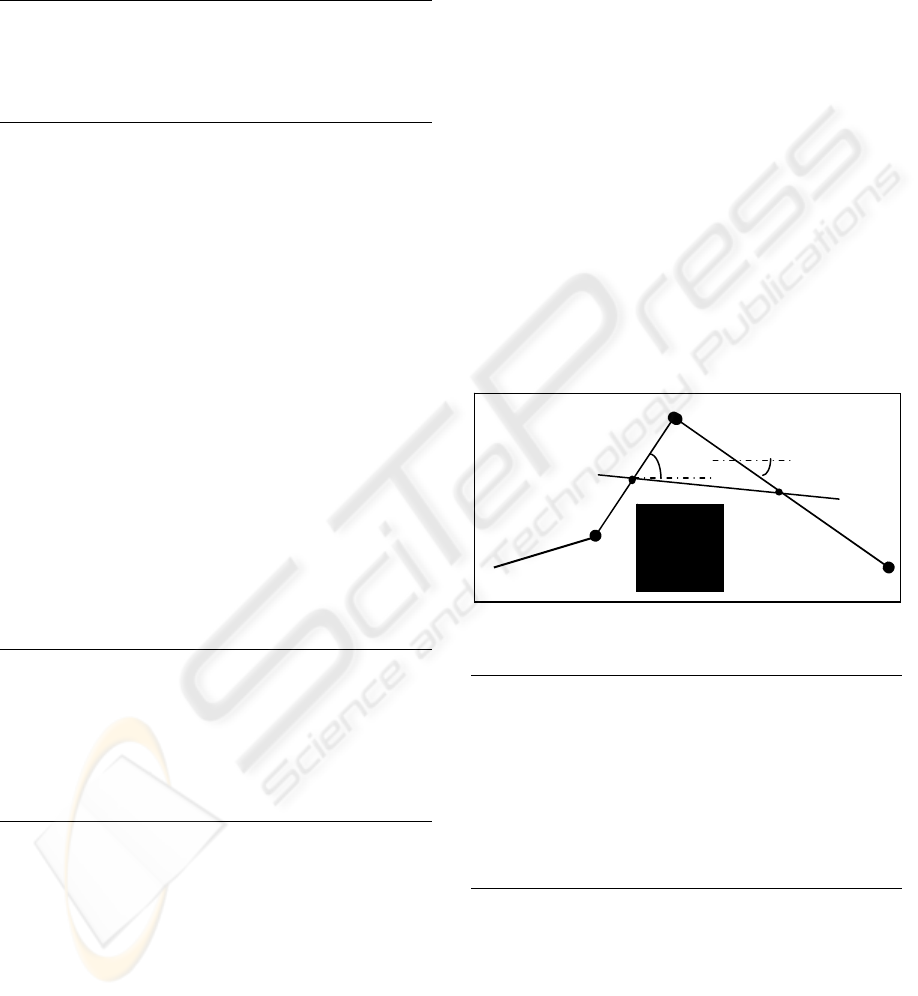
4 FINE OPTIMIZATION

Here we use a simple cut-triangle-edge scheme,

many variant are found in (Berchtold, 1994); for

each two consecutive segments E(n

) , E(n

) ,

we try to cut the triangle edge represented by n

(figure 1 ) with a segment E(n’,n”) where n’, n” are

at the middle of segment E(n

) , E(n

)

respectively .This techniques will have two

advantage:

1- Smooth the path by replacing the sharp

angles with wider ones.

2- Optimize the path in any norm (triangle’s

inequality

Cutting-tiangle-edge Algorithm

1. Input path T

2. For each segment E(n

, n

i+1

) of path T ,i=1, m-1

2.1. Calculate node n

' at the middle of segment

E(n

, n

i+1

)

3. For each segment E(n

',n'

i+1

) , i=1, m-2

3.1. If segment E(n

',n'

i+1

) is Clear

3.1.1. replace segments E(n'

, n

i+1

) and

E(n

i+1

, n'

i+1

) in T with E(n

',n'

i+1

)

4. Return T

5 CUBIC SMOOTHING

Since the PRM path are inherently peace-wise

curves. The transition from one line segment to the

next induces an abrupt change in direction. The

robot cannot execute the corresponding trajectory

without coming at rest at each of these points. In

Figure 1: cutting-triangle-edge technique

A SMOOTHING STRATEGY FOR PRM PATHS: Application to 6-axes MOTOMAN manipulator

207

order to avoid this, we should have a continuous

joint velocity. So we have to smooth path , we will

accomplish this taking care to modify the least

possible the original one, to achieve this , we smooth

the corners using a polynomial with a given degree

and parameters.

First and second order polynomial are easy to

calculate but they fit poorly, fourth order and higher

polynomials provides seamless fit but they are very

difficult if not impossible to calculate, that is why

we believe the compromise would be to choose the

cubic polynomial (Brock, 1999). The parameters are

not complicated to calculate, the curve has C

continuity and it enables tighter approximation to the

turn compared to quadratic polynomial. We will

here explain the procedure for a single joint; the

same applies to all remaining joints. The joint

position turn is governed by the following cubic

polynomial:

210

)( tatataatq +++=

(1)

The duration d of the cubic turn (Figure 2) is thus :

max





∆

(2)

Figure 2: cubic smoothing.

∆ q



is the change in velocity of the two

consecutive segments. The detailed description of

the calculation of the start and the end

configurations of the cubic turn and the cubic

parameters are found in (Brock, 1999). The Cubic

turns are tested for collision by sampling the

polynomial to a number of configuration m linearly

separated by a distance ε sufficiently small, if all m

configurations are collision free than the cubic turn

is collision free.

6 SIMULATION RESULTS

SBL planner, smoothing techniques are written in

C++, the animation and visualization API was also

implemented in C++ using COIN visualization

library and its binding SoQt.

The tests were run on a 1.7GHZ Pentium 4 PC

with 128 Mbytes of main memory running Linux

OS. We have constructed a 3D CAD model for the 6

axes MOTMAN SV3X manipulator.For the PRM

planner, the maximum number of milestones

allowed to be generated is 10000 and the distance

threshold ρ for the segment discretization was set to

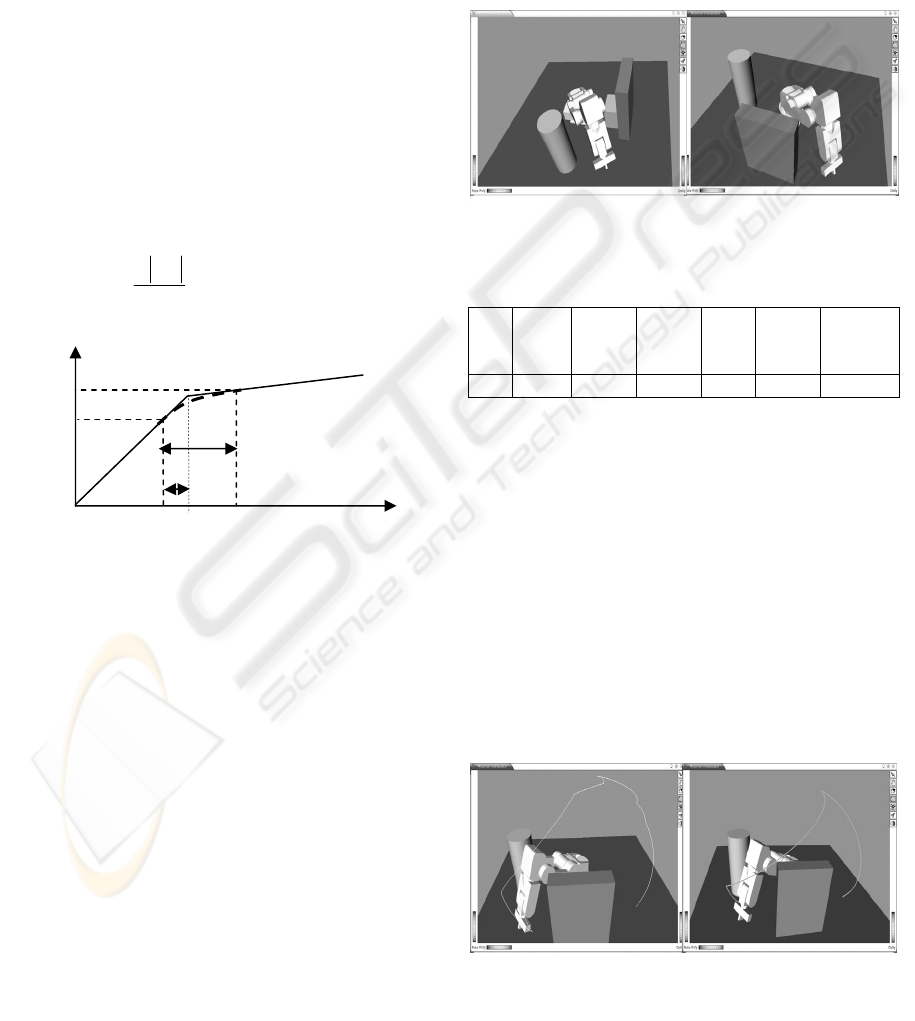
0.015. We have simulated a robot Gross movement

from initial configuration to a final configuration in

the scene shown in figure 3a, 3b respectively.

Running the SBL planner for the given query gives

the results shown in table 1.

Table 1: result of SBL planner query for the given

example.

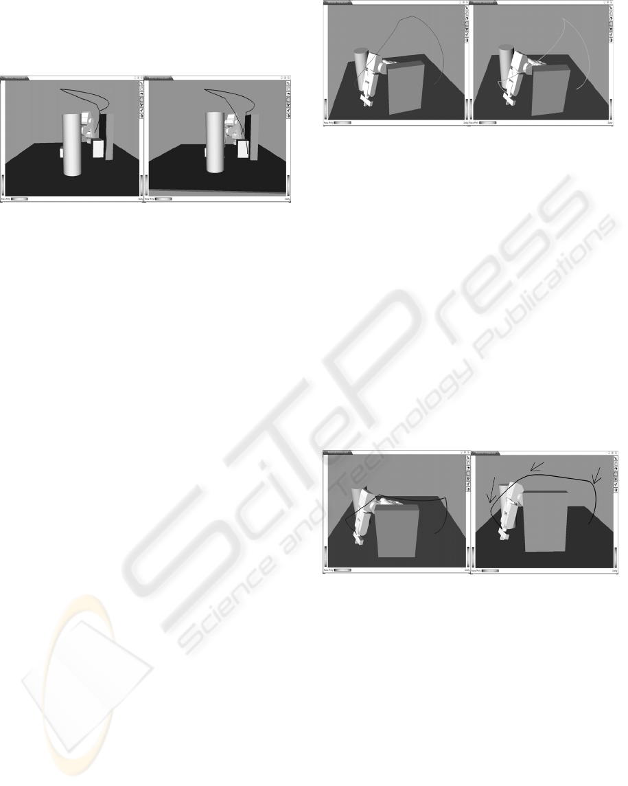
Here the generated raw path is a 7 node path,

figure 4a shows path traced by a point on the end

effector along the SBL path. It is apparent that the

path is lengthy and requires optimization.

6.1 Lazy A* application

Using a simple Euclidian path cost, the path is

shown on figure 4b with a cost of 6.66959.

If we place a weight of 10 on the shoulder axis

weighted Euclidian norm, while we put a weight on

only one, this lead to more Minimization of

Euclidian distance along that axis,. The path is

shown in figure 5a and its cost being 9.58155.

Total

-time

(s)

#nods

In trees

#nodes

In path

#total

#CC

in path

sampled

nodes

total C

time(s)

0.39

55 9 448 123 136 0.38

starting

ndi

(s)

(a) (b)

Figure 4: (a) raw trajectory, (b) Euclidian norm A* path.

(a) (b)

Figure 3: configurations, (a) initial, (b) final .

ICINCO 2005 - ROBOTICS AND AUTOMATION

208

∝

norm minimization: In this example we

penalize the maximum joint movement of the edge

between two nodes; the generated path is shown in

figure 5b with a cost of 5.7734.

a) b)

Figure 5: a) lazy A* with shoulder axis penalty path;

b) L

∝

minimization lazy A* path.

6.2 Lazy A* versus A*

In order to evaluate the efficiency of the lazy A*

with the standard A* we have run the SBL planner

for 10 times for the same query, hence 10 different

path have been generated. We have calculated the

number of collision checks required for each

technique in order to find the optimized path in some

sense. The results are:

- average Collision checks for Lazy A*: 107.7

- average Collision checks for A*: 823.4

The ratio of the two averages is ≈1/8

- Lazy A* time is = 0.25 s

- A* time is = 0.95

Using scenes that are extremely complicated will

favour more and more the use of the lazy A*

algorithm.

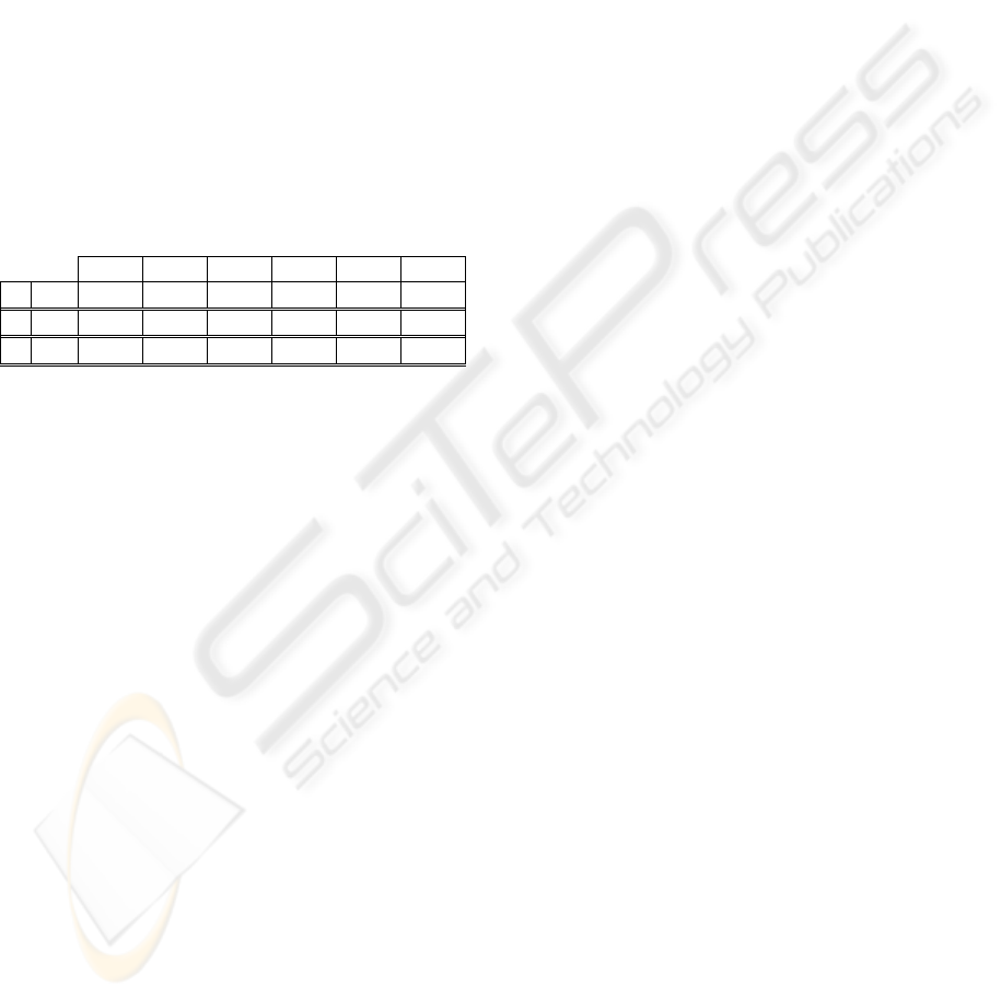
6.3 Lazy A* versus random

shortcutting

Random shortcutting (Laumond, 1990) segments

techniques are frequently used to reduce the number

of segments on the path, but the resulting path is not

necessarily optimal in any sense.

Figures 5a and 5b show the result of the

application of the Lazy A* and the Shortcutting

method respectively, in the chosen Euclidian norm,

only the A* managed to find the Optimal path, the

cost function being 6.3212, the cost for the

Shortcutting method is 7.7305.

a) b)

Figure 6: a) shortcutting path. b) Lazy A* path.

6.4 Cutting-triangle-edge

application

We apply this technique on the optimal A* path

(figure 4b), it is clear that the application of this

technique will not dwarf any optimization gained

from the A* because it only shortcut parts of

segments which is more optimized in any norm used

(this is the triangle’ inequality which is a condition

of normality).

The results are:

- the algorithm managed to cut all segment

- the cost of path generated is : 5.77343

- the time taken is : 0.05 seconds

Figure 7a shows the generated path.

a) b)

Figure 7: a) cutting-triangle-edge path: b) cubic smoothing

path.

6.5 Cubic smoothing and trajectory

generation

Up to now, we where dealing with C-space spatial

paths, in order to execute the path parameterized

with time or simply the trajectory, we need to

associate joint velocities with each segment of the

path. It is clear that if we require the robot to follow

a C-space straight line segment of the path, then we

should synchronize all joints with constant velocities

so that the joint movement is linear.

What we have done is chose a velocity v that is

smaller or equal than any of the physical maximum

joint velocities. v is fixed for all segments making

A SMOOTHING STRATEGY FOR PRM PATHS: Application to 6-axes MOTOMAN manipulator

209

the path. Using v and the maximum joint

displacement in the given segment, we calculate the

segment duration d

, d

is used to calculate the joint

velocities for the remaining 5 joints. In this way, we

guarantee our piece-wise path following and prevent

assigning later joint velocities that exceed actual

ones.

Choosing v to be 0.10s

-1

, we calculated the 6

joints velocities and durations for all 4 segments

making the path issued from the fine optimization

step (figure 7a).

The total duration of the trajectory is 9.6246

seconds. Using this trajectory along with typical

maximum normalized acceleration of 0.20s

-2

calculated the 3 cubic durations and polynomial’s

parameters. Table 2 shows the calculated cubic

durations for the three corners smoothed.

Figure 7b shows the path with smoothed corners.

Table 2: cubic smoothing durations

d(s)

0.1851

0.3350

0.1122

0.0125

0.1466

d(s)

0.2867

1.3977

0.1125

0.0462

0.1749

1.0765

d(s)

0.4878

0.1580

0.4982

0.1064

0.5288

0.9235

The cubic duration that is null means no cubic

turn is needed due to the velocities of the two

consecutive segments being equal. It is clear that the

total trajectory duration can be reduced by using

higher joint velocities, but the cubic deviation will

be consequently higher.

7 CONCLUSION AND FUTURE

WORKS

The results show that the PRM paths can be

optimized through any criterion thought the Lazy A*

algorithm instead of blind shortcutting techniques,

the proposed lazy A* calculate the optimal path with

minimum collision checks compared to standard A*,

the remaining edges are smoothed thought cubic

polynomial resulting in minimum deviation from

original path, the final trajectory is an optimized

smooth trajectory ready for execution.

We are implementing the approach on the

physical MOTOMAN SV3X 6-axes manipulator,

and also working on a scheme to optimize

furthermore the PRM path by using an enhanced A*

algorithm along with other techniques.

REFERENCES

Latombe J-C., 1991. Robot Motion Planning, Kluwer

Academic Publishers.

Kavraki, E., Svestka, P., Latombe, J-C. and Overmars,

M.H, 1996. Probabilistic Roadmap for path planning in

high-dimensional configuration spaces, IEEE Trans,

Robot & Autom, 12(4) 556-580.

Lozano-Péerez, T. and Wesley, M.A, 1979. An Algorithm

for Planning Collision Free Paths among Polyhedral

Obstacles, Communications of the ACM, vol. 22 ,no.

10, pp. 560-570.

Larsen, E., Gottschalk, S., Lin, M-C., Manocha, D., 1998.

Fast Proximity Queries with Swept Sphere Volume»,

Technical report TR99-018, Department of Computer

Science, University of N. Carolina, Chapel Hill.

Sanchez-Ante, G. and Latombe, J-C., 2001. A single-

query bi-directional probabilistic roadmap planner with

lazy collision checking, In Proc, 10th Int. Symp. Of

Robotics Research, ISRR’2001, Lorne, Victoria,

Australia.

Bohlin, R. and Kavraki, L., 2000. Path Planning Using

Lazy PRM. In Proceedings of the IEEE International

Conference on Robotics and Automation, pp. 521–528,

IEEE Press, San Fransisco, CA.

Quinlan, S. and Khatib, O., 1993. Elastic Bands:

Connecting Path Planning and Control,’’ Proceedings

of the International Conference on Robotics and

Automation, Atlanta, GA, pp. 802-807.

Foley, J., van Dam, A., Feiner, S. and Hughes,. J. 1990

Computer Graphics: Principles and Practices, 2nd ed.

Addison-Wesley.

Kant, K. and Zucker. S-W. 1987. Planning smooth

collision-free trajectories: path, velocity, and splines in

free-space,” The International Journal of Robotics

Research, 2(3), pp.117–126.

Tondu, B. and Bazaz, S.A. 1999. The Three-Cubic

Method: An Optimal Online Robot Joint Trajectory

Generator under Velocity, Acceleration, and

Wandering Constraints,” The International Journal of

Robotics Research, vol.18, n°9 pp.893–901.

Laumond, J-P. Taix, M. and Jacobs, P. 1990. A motion

planner for car-like robots based on a global/local

approach," Proc. IEEE Internat. Workshop Intell.

Robot Syst. 765-773.

Berchtold, S. and Glavina, B., 1994. A scalable optimizer

for automatically generated manipulator motions, Proc.

IEEE/RSJ/GI Int. Conf. Intelligent Robots and

Systems, 1796-1802, München, Germany.

Doyle, A-B., 1995. Algorithms and Computational

Techniques for Robot Path Planning”, Phd thesis.

Brock, O., 1999. Generating robot motion; the integration

of planning and execution, PhD thesis, Stanford

University.

ICINCO 2005 - ROBOTICS AND AUTOMATION

210