SUNSPOT SERIES PREDICTION USING ADAPTIVE
IDENTIFICATION
Juan A. Gómez Pulido, Miguel A. Vega Rodríguez, José Mª Granado Criado, Juan M. Sánchez Pérez
Departament of Computer Sciences, University of Extremadura, Spain
Keywords: System Identification. Prediction. Solar series. Parallelism.
Abstract: In this paper a parallel and adaptive methodology for optimizing the time series prediction using System
Identification is shown. In order to validate this methodology, a set of time series based on the sun activity
measured during the 20th century have been used. The prediction precision for short and long term
improves with this technique when it is compared with the found results using System Identification with
classical values for the main parameters.
1 INTRODUCTION
The time series (TS) prediction is a very important
knowledge area because the evolution of many
processes is represented as a time series:
meteorological phenomena, chemical reactions,
financial indexes, etc. Although the behaviour of any
of these processes may be due to the influence of
several causes, in many cases the ignorance of these
forces to study the process considering only the time
series evolution that represent it. By this reason,
numerous methods of time series analysis and
mathematical modelling have been developed.
System Identification (SI) techniques
(Söderström, 1989) can be used to obtain the TS
model. The model precision depends on the assigned
values to certain parameters. In SI, a time series is
considered as a sampled signal y(k) with period T
that is modeled with an ARMAX (Ljung, 1999)
parametric polynomial description of na dimension.
Basically the identification consists in determining
the ARMAX model parameters from measured
samples. Then it is possible to compute the
estimated signal ye(k) and to compare it with the
real signal, calculating the error (y(k)-ye(k)).
The recursive estimation updates the model in
each time step k, thus modeling the system. The
more sampled data are processed, the more precision
for the model, because it has more information about
the system behaviour history. We consider SI
performed by the well-known Recursive Least
Squares (RLS) algorithm (Ljung, 1999). This
algorithm is mainly specified by the constant λ
(forgetting factor) and the observed samples {y(k)}.
There is not any fixed value for λ, even it is used a
value between 0.97 and 0.995 (Ljung, 1991). The
cost function F we use is defined as the value to
minimize in order to obtain the best precision (see
equation 1, where SN is the sample number).
F(λ) =
Equation 1: The considered cost function
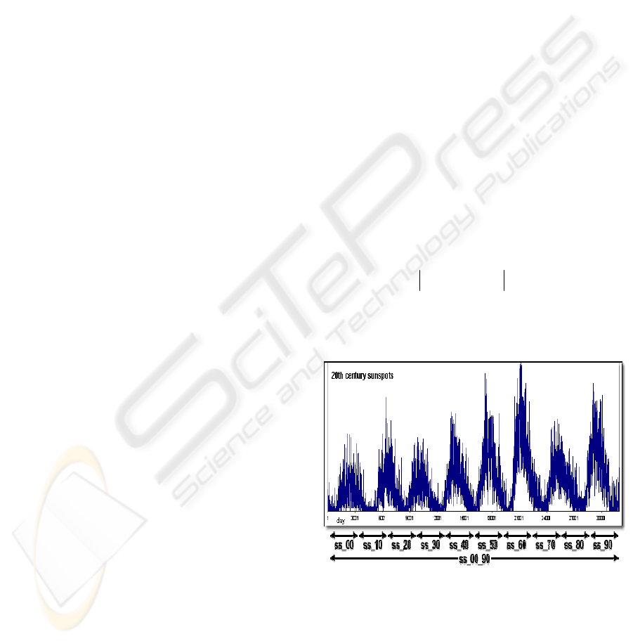
Figure 1: The sunspot time series used in this work
In this paper we use a time series set
corresponding to sunspot series obtained from
measured observations (ROB, 2004)(NOAA, 2004).
We have used 13 time series (Fig. 1) showing daily
sunspots: ten series (ss_00, ss_10, ss_20, ss_30,
ss_40, ss_50, ss_60, ss_70, ss_80 and ss_90)
corresponding to the sunspot measurements during
∑
− yy
−+=
=
1
0
0
)()(
SNkk
kk
e
kk
224
A. Gómez Pulido J., A. Vega Rodríguez M., M
a
Granado Criado J. and M. Sánchez Pérez J. (2005).
SUNSPOT SERIES PREDICTION USING ADAPTIVE IDENTIFICATION.
In Proceedings of the Second International Conference on Informatics in Control, Automation and Robotics - Signal Processing, Systems Modeling and
Control, pages 224-228
DOI: 10.5220/0001166202240228
Copyright
c
SciTePress
ten years each (for example, ss_20 compiles the
sunspots from 1/1/1920 to 31/12/1929), two series
(ss_00_40 and ss_50_90) covering 50 years each,
and finally one series (ss_00_90) that covers all
measurements of the 20th century.
2 SYSTEM IDENTIFICATION
BASED PREDICTION
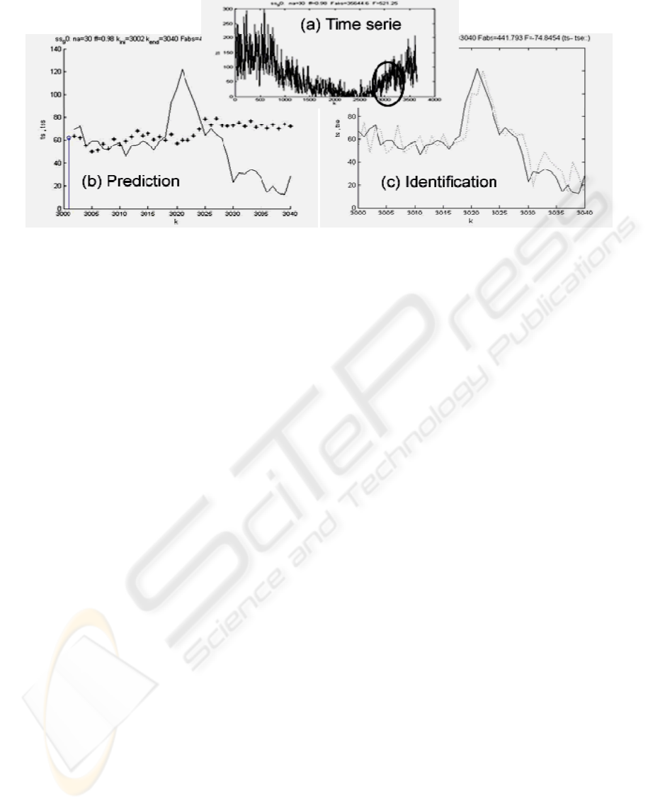
The recursive identification can be used to predict
the following behaviour of the time series (Fig. 2a)
from the data observed up to the moment. It is well
known that SI allows finding, in sample time, a
mathematical model of a system in the k time from
which is possible to predict the system behaviour in
k+1, k+2 and so on. As identification advances in
the time, the predictions improve using more precise
models. If ks is the time until the model is elaborated
and from which we carry out the prediction, we can
confirm that this prediction will have a larger error
while we will be more far away from ks (Fig. 2b).
The predicted value for ks+1 corresponds with the
last estimated value until ks. When we have more
data, the model starts to be re-elaborated for
computing the new estimated values (Fig. 2c).
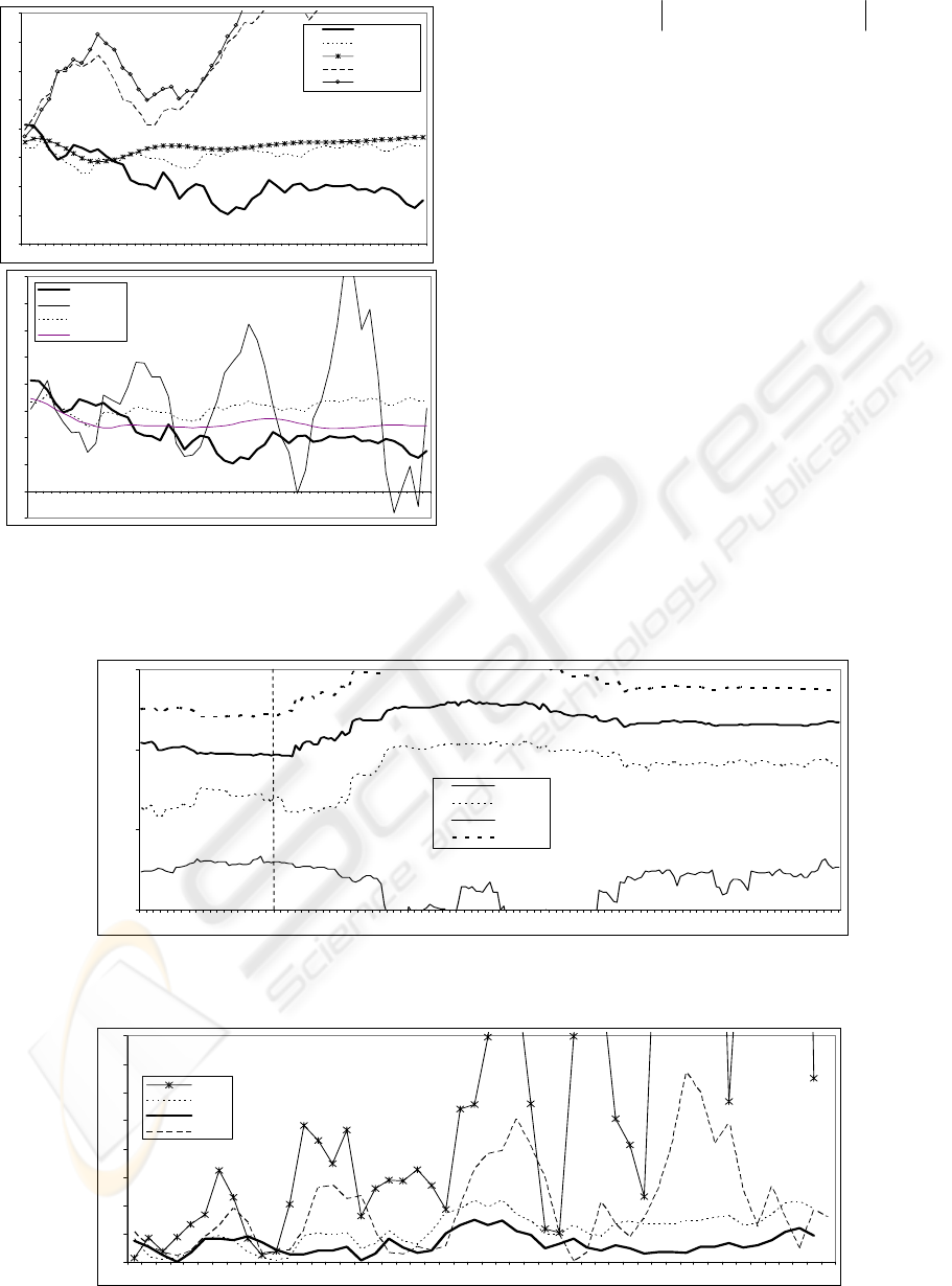
The main parameters of the identification are na y
λ. Both parameters have influence on the precision
of prediction results, as it shows Fig. 3. As we can
see, to establish an adequate value of na and λ may
be critical in order to obtain a good prediction. By
this reason, in the strategy of optimizing the
prediction, we try, first of all, to establish an
adequate dimension of the mathematical model for
finding the optimal λ value using an adaptive
algorithm.
In order to do that, many experiments have been
carried out. In these experiments, the absolute
difference between the real and predicted values has
been used in order to quantify the prediction
precision (see equation 2). So, in Fig. 4 the results of
many experiments are shown. In these experiments
different measures of the prediction error (for short
term DIFA1 and for long term DIFA50) for 200
different values of the model are obtained. In order
to establish reliable conclusions, these experiments
have been made for different ks values.
Figure 2: In (a) is displayed the ss_90 series. If ks=3000, we can see in (b) the long-term prediction based on the model
obtained up to ks (na=30 and λ=0.98). The prediction precision is reduced when we are far from ks. In (c) we can see the
predicted values for the successive ks+1 obtained from the updated models when the identification (and ks) advances
We use our own terminology for the prediction
error (DIFAX, where X is an integer) because like
this the reader can understand more easily the degree
of accuracy that we are measuring.
Provisionally we conclude that the increase of na
does not imply an improvement of the prediction
precision (however a considerable increase of the
computational cost is spent). This is easily verified
using large ks values (the elaborated models have
more information related to the time series) and
long-term predictions. From these results and as
trade-off between prediction and computational cost,
we have chosen na=40 to establishing it as the model
size for the future experiments
SUNSPOT SERIES PREDICTION USING ADAPTIVE IDENTIFICATION
225
DIFA(X) =
na influe nce (ff=0.98, ks=3600)
0
50
Figure 3: Influence of the model dimension na and
forgetting factor λ on the short-term (ks) and long-term
(ks+50) prediction for the ss_90 series
Eq.2. The cost function in the prediction
measurements.
The key parameter for the prediction optimization
is λ. Fig. 5 shows, with more detail than in Fig. 3b,
an example of the λ influence in the short-term and
long-term predictions by representing its precision
measure. It is clear that for any λ value is more
precise the short-term prediction than the long-term
prediction. However, we can observe the chosen
value for λ is critical for finding a good predictive
model (from the four chosen values, λ =1 produces a
better prediction, even in the long term). This
analysis has been confirmed making a great number
of experiments with the sunspot series, modifying
the initial prediction time, ks.
Figure 4: Measures of the prediction precision for the ss_90 time series from ks=3600, using λ=0.98. The measures have
been made for models of dimensions between 2 and 200
.
Figure 5: Influence of λ in the prediction precision for ss_90 with na=40 and ks=3600
100
0
0
0
0
0
0
ks+1 ks+8 ks+15 ks +22 ks +29 ks+36 ks +43 ks +50
40
35
30
25
20
15
ts
tss (na=40)
tss (na=10)
tss (na=75)
tss (na=100)
FF influence (na =40, ks=3600)
-50
0
50
100
150
200
250
300
350
400
ks+1 ks+8 ks+15 ks+22 ks+29 ks+36 ks +43 ks+50
ts
ts s (ff=0.95)
ts s (ff=0.98)
tss (ff=1)
10
100
1000
10000
2 13 24 35 46 57 68 79 90 101 112 123 134 145 156 167 178 189 200
na
log10
DIFA 1
DIFA 10
DIFA 25
DIFA 50
DIFA(X)
(na = 40, ks=3600)
0
50
100
150
200
250
300
350
400
1 8 15 22 29 36 43 50
X
ff=0.9
ff=0.98
ff=1.0
ff=0.95
∑
=
=
+−+
Xi
i
s
iksyiksy
1
)()(
ICINCO 2005 - SIGNAL PROCESSING, SYSTEMS MODELING AND CONTROL
226
3 OPTIMIZING THE
PREDICTION WITH AN
ADAPTIVE STRATEGY
In order to find the optimum value of λ, we propose
an adaptive algorithm inspired on the artificial
evolution (Goldberg, 1989)(Rechenberg, 1973) and
on the simulated annealing mechanism (Kirkpatrick,
1983). This algorithm, named PARLS (Parallel
Adaptive Recursive Least Squares), has been
implemented using parallel processing units, built
with neural networks (Gomez, 2003). In PARLS the
optimization parameter λ evolves to predict new
situations during the iterations of the algorithm. In
other words, λ evolves at the same time that
improves the cost function performance.
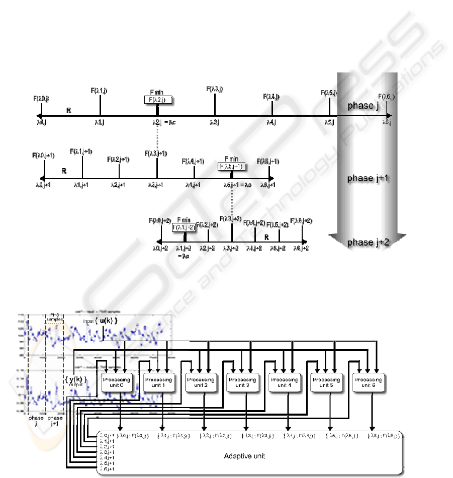
The evolution mechanism (Fig. 6) is as follows:
The first phase starts building a set of λ values
covering the interval R uniformly from its selected
middle λc. An equal number of parallel processing
units (PUN) perform RLS identification with each λ
in the interval, for a given number of sampling times
(PHS). Then, the optimum λ is that whose
corresponding cost function F is the minimum of all
computed F, and from it a new set of λ values is
generated and used in the next phase to perform new
identifications during the following PHS samples. F
is defined as the accumulated error of the samples in
each phase, and the generation of new λ values is
made with a more reduced R by the factor RED.
Finally, PARLS stops when the number of phases
(PHN) is reached, according to the total number of
samples (TSN).
Figure 6: All the λ values in the same phase running in the processing units are generated in the R interval from the
previous phase optimum λ found, corresponding with the smallest F
.
Figure 7: PARLS architecture. A set of processing units generates the next set of λ values to be computed by RLS algorithm
SUNSPOT SERIES PREDICTION USING ADAPTIVE IDENTIFICATION
227

Therefore, PARLS could be considered as a
population-based rather than a parallel
metaheuristic, because each processing unit is able
to operate isolated, as well as the tackled problem
itself as only a single real-valued parameter (λ) that
is optimized.
In Fig. 7 we can see a top-level view of the
PARLS architecture: a set of processing units that
performs system identification in each phase sends
the errors found to the adaptive unit. This unit will
generate the new search range in a feedback loop.
4 EXPERIMENTAL RESULTS
Some results found using the PARLS algorithm for
predicting the next values from the last value
registered for the time series of the sun activity
indexes of the 20th century second half are shown in
Table 1. The prediction precision is given by the
results DIFA1 (short term) and DIFA50 (long term).
These results are compared, for evauating purposes,
with the obtained using RLS identification with
some values of λ inside the classical range (Ljung,
1991). We can see how PARLS finds a better
precision.
5 CONCLUSIONS
The results shown in Table 1 are a part of the great
number of experiments carried out using different
time series and initial prediction times. In the great
majority of the cases, PARLS offers better results
than if λ random values are used. However, we are
trying to increase the prediction precision. Thus, our
future working lines suggest using genetic
algorithms or strategies of analogous nature for, on
the one hand, finding the optimum set of values for
the parameters of PARLS and, on the other hand,
finding the optimum couple of values {na, λ}.
ACKNOWLEDGEMENTS
This work has been developed thanks to TRACER
project, TIC2002-04498-C05-01.
REFERENCES
Söderström, T. et al., 1989. System Identification.
Prentice-Hall, London.
Ljung, L., 1999. System Identification – Theory for the
User. Prentice-Hall, London.
Ljung, L., 1991. System Identification Toolbox. The Math
Works Inc, NY.
ROB, Royal Observatory of Belgium, Brussels, 2004.
Sunspot Data Series. http: // sidc.oma.be / html /
sunspot.html
NOAA, National Geophysical Data Center, 2004. Sunspot
numbers. http: // www. ngdc. noaa.gov / stp / SOLAR /
ftpsunspotnumber.html
Goldberg, D.E., 1989. Genetic Algorithms in Search,
Optimization and Machine Learning. Addison Wesley.
Rechenberg, I., 1973. Evolutionsstrategie: Optimierung
technischer systeme nach prinzipien der biolgischen
evolution. Formmann-Holzboog Verlag.
Kirkpatrick, S., Gelatt, C., Vecchi, M., 1983. Optimization
by Simulated Annealing. In: Science, 220, 4598, 671-
680.
Gómez, J., Sánchez, J., Vega, M., 2003. Using Neural
Networks in a Parallel Adaptive Algorithm for the
System Identification Optimization. In: Lecture Notes
on Computer Sciences, vol. 2687, 465-472. Springer-
Verlag.
Table 1: A sample of the prediction precision results for short and long term, compared with the ones obtained from
three classical values of λ: 0.97, 0.98 and 0.995. The settings for this experiment are: benchmark= ss_50_90; na=40;
ks=18,210; TSN=18,262; λc=1; R=0.2; RED=2
ICINCO 2005 - SIGNAL PROCESSING, SYSTEMS MODELING AND CONTROL
228
