ANALYSIS AND SYNTHESIS OF DIGITAL STRUCTURE BY
MATRIX METHOD
B. Psenicka
Universidad Nacional Autonoma de M
´
exico
R. Bustamante Bello
TEC de Monterey,Campus Ciudad de M
´
exico
M.A.Rodriguez
Universidad Polit
´
ecnica de Valencia
Keywords:
Synthesis, Analysis, Digital structures, Algorithm, Matrix Method.
Abstract:
This paper presents a general matrix algorithm for analysis and synthesis of digital filters. A useful method
for computing the state-space matrix of a general digital network and a new technique for the design of digital
filters are shown by means of examples. The method proposed in this paper allows the analysis of the digital
filters and the construction of new equivalent structures of the canonic and non canonic digital filter forms.
Equivalent filters with different structures can be found according to various matrix expansions. The procedure
proposed in this paper is more efficient and economic than traditional methods because it permits to construct
circuits with a minimum of shifting operations.
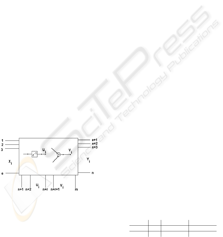
1 INTRODUCTION
The digital system presented in figure 1 is described
by the following equations:
Figure 1: State-space structure with multiple inputs and out-
puts.
Y(z)= F
YX
X(z)+F
YU
U(z)+F
YV
V(z)
U(z)= F
UX
X(z)+F
UU
U(z)+F
UV
V(z)
V(z)= F
VX
X(z)+F
VU
U(z)+F
VV
V(z)
(1)
or in matrix form (2), (Luecker, 1976)
N
s
×
⎡
⎢
⎣
X(z)
Y(z)
U(z)
V(z)
⎤
⎥
⎦
= 0, (2)
where N
s
in equation (2) is the signal flow matrix that
represents the signal-flow graph of the digital system
with multiple inputs and multiple outputs, X(z) is the
vector of the input signals X
i
, Y(z) is the vector of
the output signals Y
i
, U(z) is the vector of the signals
U
i
in the output of the delay elements and V(z) is a
vector of the signals V
i
in the output of the adders,
see figure 1. N
s
can be obtained by expression (3),
where F
YX
in the equation (3) is the transfer matrix
output/input, F
YX
= Y(z)/X(z) if U(z)=V(z)=0. In
figure 2, signals U
3
and U
4
represent the outputs of
the delay elements and signals V
5
and V
6
designate
the outputs of the summers.
N
s
=
⎡
⎣
F
(YX
) −E F
(YU)
F
(YV)
F
(UX)
0 F
(UU)
− E F
(UV )
F
(VX)
0 F
(VU)
F
(VV)
− E
⎤
⎦
(3)
If we reduce the signals avoiding the outputs of the
adders V
i
in expression (2), we obtain
22
Psenicka B., Bustamante Bello R. and A. Rodriguez M. (2005).
ANALYSIS AND SYNTHESIS OF DIGITAL STRUCTURE BY MATRIX METHOD.
In Proceedings of the Second International Conference on Informatics in Control, Automation and Robotics - Signal Processing, Systems Modeling and
Control, pages 22-29
DOI: 10.5220/0001165200220029
Copyright
c
SciTePress

N
e
×
X(z)
Y(z)
U(z)
= 0, (4)
where N
e
in equation (4) is a flow-state matrix and
the matrices A, B, C and D in the matrix equation
(5) are the state matrices of the digital system.
N
e
=
D
−E C
z
−1
B 0 z
−1
A − E
(5)
In the flow-state matrix, the matrices E and 0 are
identity and zero matrices respectively. If we reduce
the matrix equation (4), not taking into account the
vector of the signals U
i
, we get the expression
N
(2)
t
×
X(z)
Y(z)
= 0, (6)
where the transfer matrix N
(2)
t
can be defined by (7)
N
(2)
t
=
D + C × (zE − A)
−1
B; −E
(7)
The element n
(2)
21
of the transfer matrix N
(2)
t
is the
transfer function H(z) of the digital network.
n
(2)
21
= H(z)=D + C × (zE − A)
−1
B (8)
Using the inverse z transform, the impulse response
of the circuit results (Luecker, 1976)
h(n)=
⎧
⎨
⎩
D for l =0
CA
l−1
B for l > 0
(9)
where l=1,2,3 ...
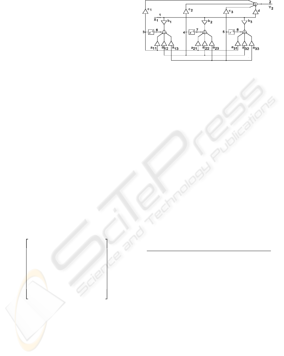
2 ANALYSIS OF THE SECOND
ORDER STATE-SPACE DIGITAL
FILTER
As an example, we will determine the transfer func-
tion of a state-space second order digital filter, see fig-
ure 2. To calculate the signal-flow matrix of the digi-
tal filter, previously it is necessary to mark the input,
output and state nodes (P
ˇ
seni
ˇ
cka and Herrera, 1997),
(P
ˇ
seni
ˇ
cka and Ugalde, 1999). The input node is de-
noted by number 1 and the output node by number 2.
The nodes 3 and 4 are assigned to the outputs of the
delay elements. Finally, the nodes 5 and 6 are placed
on the output of the adders. The system equations
(10) for each node can be obtained from figure 2.
Figure 2: State-space digital filter of second order.
2:Y
2
= X
1
d + U
3
c
1
+ U
4
c
2
3:U
3
= V
6
z
−1
4:U
4
= V
5
z
−1
5:V
5
= X
1
b
2
+ U
3
a
21
+ U
4
a
22
6:V
6
= X
1
b
1
+ U
3
a
11
+ U
4
a
12
(10)
The equations (10) can be written by the matrix equa-
tion to generate the signal flow matrix N
(6)
s
. The first
row of the matrix (11) is indexed by number 2, see
also expression (10).
123 4 5 6
N
(6)
s
=
2
3
4
5
6
⎡
⎢
⎢
⎢
⎣
d −1 c
1
c
2
00
00−10 0z
−1
00 0−1 z
−1
0
b
2
0 a
21
a
22
−10
b
1
0 a
11
a
12
0 −1
⎤
⎥
⎥
⎥
⎦
(11)
From the signal-flow matrix (11)we can observe, that
the main diagonal contain -1’s and in the second col-
umn all the elements are zeros except the first one.
The signal-flow matrix can be formed directly with-
out writing node equations (10). For example, due
to the delay element placed between the nodes 6 and
3, see figure 2, the matrix element n
(6)
36
of the matrix
N
(6)
s
acquires the value z
−1
. The multiplier a
21
lo-
cated between the nodes 3 and 5 is represented in the
matrix N
(6)
s
by the element n
(6)
53
equal to the constant
a
21
. Similarly, we can obtain all of the elements in
the signal-flow matrix without writing the nodal equa-
tions. The matrix N
(6)
s
can be reduced to the matrix
N
(5)
equation (13) according to the expression
n
(k−1)
ij
=
n
(k)
ij
n
(k)
kk
− n
(k)
ik
n
(k)
kj
n
(k)
kk
, (12)
where i represents the number of the row, j the number
of the column and k the degree of the matrix.
ANALYSIS AND SYNTHESIS OF DIGITAL STRUCTURE BY MATRIX METHOD
23

Following the rule of reduction (12), we obtain the
matrix N
(5)
and the state-flow matrix N
(4)
e
N
(5)
=
⎡
⎢
⎣
d −1 c
1
c
2
0
z
−1
b
1
0 −1+a
11
z
−1
a
12
z
−1
0
00 0 −1 z
−1
b
2
0 a
21
a
22
−1
⎤
⎥
⎦
(13)
N
(4)
e
=
⎡
⎣
d
−1 c
1
c
2
z
−1
b
1
0 −1+a
11
z
−1
a
12
z
−1
z
−1
b
2
0 a
21
z
−1
−1+a
22
z
−1
⎤
⎦
(14)
If we compare the expressions (14) and (5), we obtain
the state matrices A, B, C, and D of the state-space
digital filter.
D = d C =[
c
1
c
2
]
B =
b
1
b
2
A =
a
11
a
12
a
21
a
22
(15)
3 DESIGN OF THE THIRD
ORDER STATE-SPACE
STRUCTURE
In this example we are going to obtain the third order
state-space structure. The state matrices of the third
order state-space filter have the general form (16),
(Psenicka et al., 1998).
D = d C =[
c
1
c
2
c
3
]
B =
b
1
b
2
b
3
A =
a
11
a
12
a
13
a
21
a
22
a
23
a
31
a
32
a
33
(16)
Substituting (16) in (5) it is obtained the state-flow
matrix (17)
N
(5)
e
=
⎡
⎢
⎢
⎢
⎣
d −1 c
1
c
2
c
3
z
−1
b
1
0 −1+a
11
z
−1
a
12
z
−1
a
13
z
−1
z
−1
b
2
0 a
21
z
−1
−1+a
22
z
−1
a
23
z
−1
z
−1
b
3
0 a
31
z
−1
a
32
z
−1
−1+a
33
z
−1
⎤
⎥
⎥
⎥
⎦
(17)
To expand the state-flow matrix (17) which contains
five columns and four rows in the matrix with six
columns and five rows (19) , we use the equation (18).
The equation (18) is obtained from equation (12) for
n
(k)
kk
= −1.
n
(k)
ij
= n
(k−1)
ij
− n
(k)
ik
n
(k)
kj
(18)
If we choose the elements of the new matrix n
(6)
26
=
n
(6)
46
= n
(6)
56
=0, then the first, third and fourth rows
in the new matrix N
(6)
remain unchanged (19).
N
(6)
=
d −1 c
1
c
2
c
3
0
n
(6)
31
n
(6)
32
n
(6)
33
n
(6)
34
n
(6)
35
n
(6)
36
z
−1
b
2
0 a
21
z
−1
−1+a
22
z
−1
a
23
z
−1
0
z
−1
b
3
0 a
31
z
−1
a
32
z
−1
1 − a
33
z
−1
0
n
(6)
61
n
(6)
62
n
(6)
63
n
(6)
64
n
(6)
65
n
(6)
66
(19)
The elements of the matrix (19), n
(6)
61
,n
(6)
62
,n
(6)
63
,
n
(6)
64
,n
(6)
65
,n
(6)
66
and n
(6)
36
can be chosen and the re-
maining elements n
(6)
31
,n
(6)
32
, n
(6)
33
,n
(6)
34
and n
(6)
35
are
obtained by means of the equation (18). The elements
in the last row and columns of the matrix N
(6)
must
be chosen, in order to obtain in the second row of the
matrix N
(6)
plenty of zeros. It is suitable to choose
the element n
(6)
36
= z
−1
, because all elements in the
second row of the matrix N
(5)
e
contain z
−1
. But it is
possible select the element n
(6)
36
in a different way, as
we shall see in section 4.2. If we choose
n
(6)
26
=0 n
(6)
46
=0 n
(6)
56
=0 n
(6)
62
=0
n
(6)
66
= −1 n
(6)
65
= a
13
n
(6)
64
= a
12
n
(6)
63
= a
11
n
(6)
36
= z
−1
n
(6)
61
= b
1
then we get by equation 18 the elements of the new
matrix in the form
n
(6)
31
= n
(5)
31
− n
(6)
36
n
(6)
61
= z
−1
b
1
− z
−1
b
1
=0
n
(6)
32
= n
(5)
32
− n
(6)
36
n
(6)
62
=0− z
−1
0=0
n
(6)
33
= n
(5)
33
− n
(6)
36
n
(6)
63
= −1+a
11
z
−1
− a
11
z
−1
= −1
n
(6)
34
= n
(5)
34
− n
(6)
36
n
(6)
64
= z
−1
a
12
− z
−1
a
12
=0
n
(6)
35
= n
(5)
35
− n
(6)
36
n
(6)
65
= z
−1
a
13
− z
−1
a
13
=0
and we obtain the matrix N
(6)
N
(6)
=
d −1 c
1
c
2
c
3
0
00−10 0z
−1
z
−1
b
2
0 a
21
z
−1
−1+a
22
z
−1
a
23
z
−1
0
z
−1
b
3
0 a
31
z
−1
a
32
z
−1
−1+a
33
z
−1
0
b
1
0 a
11
a
12
a
13
−1
(20)
ICINCO 2005 - SIGNAL PROCESSING, SYSTEMS MODELING AND CONTROL
24
Similarly, we can obtain the matrices N
(7)
and N
(8)
.
After a very simple calculation, we can get the matrix
(21) and the signal-flow matrix (22). For example it
is advantageous to choose the element n
(7)
47
= z
−1
,in
the matrix N
(7)
, because each element in row 3 of the
matrix N
(6)
contains z
−1
. In case the matrix element
n
(7)
71
equal to b
2
is chosen, the element n
(7)
41
is equal
to zero, marked by |0|. For example in order to obtain
in the matrix N
(7)
n
(7)
41
=0if n
(6)
41
= b
2
· z
−1
it is
necessary to choose n
(7)
47
= z
−1
and n
(7)
71
= b
2
or
viceversa. So to obtain in the matrix N
(8)
n
(8)
55
= −1
if n
(7)
55
= −1+a
33
· z
−1
it is necessary to choose
n
(8)
58
= z
−1
and n
(8)
85
= a
33
or the contrary. The same
procedure can be applied to equation (21) in order to
get equation (22).
N
(7)
=
⎡
⎢
⎢
⎢
⎢
⎢
⎢
⎢
⎢
⎣
d −1 c
1
c
2
c
3
00
00−10 0 z
−1
0
|0| 00 −100|z
−1
|
z
−1
b
3
0 a
31
z
−1
a
32
z
−1
−1+a
33
z
−1
00
b
1
0 a
11
a
12
a
13
−10
|b
2
| 0 a
21
a
22
a
23
0 −1
⎤
⎥
⎥
⎥
⎥
⎥
⎥
⎥
⎥
⎦
(21)
N
(8)
=
d −1 c
1
c
2
c
3
000
00−10 0z
−1
00
00 0 −10 0z
−1
0
00 0 0 −10 0z
−1
b
1
0 a
11
a
12
a
13
−10 0
b
2
0 a
21
a
22
a
23
0 −10
b
3
0 a
31
a
32
a
33
00−1
(22)
The digital structure that corresponds to the signal
flow matrix N
(8)
is presented in figure 3.
The second canonic form of the state-space digital fil-
ter can be obtained from the structure presented in
figure 3. Changing the adders to nodes, the nodes
to adders, the input to output and the directions of
the multipliers, the second canonic form of the state-
space filter can be obtained. If other values are cho-
sen for elements in the last row and the last column
in matrices (19), (20) and (21) we can obtain other
equivalent structure.
Figure 3: Third order state-space filter.
4 EXAMPLES
4.1 Design of the filter from the state
space matrices
In the first example we shall demonstrate how to de-
rive the structures of the state-space filter without
multipliers if the state-space matrices A, B, C and
D are known (23).
D =0.25 C =[
0.25 0.5
]
B =
0.75
0.75
A =
−0.5 −0.5
0.50.5
(23)
With the assistance of equation (5) we obtain the
state-space matrix N
(4)
e
in the form
N
(4)
e
=
⎡
⎢
⎣
2
−2
−12
−2
2
−1
(2
−2
+2
−1
)z
−1
0 −1+2
−1
z
−1
2
−1
z
−1
(2
−2
+2
−1
)z
−1
02
−1
z
−1
−1+2
−1
z
−1
⎤
⎥
⎦
(24)
Provided that we choose elements n
(5)
ij
in the matrix
N
(5)
in this way n
(5)
25
=0, n
(5)
35
= z
−1
, n
(5)
45
=0
and n
(5)
55
= −1 we obtain the equation (25) from the
equation (24). In the new matrix N
(5)
the elements
in the last row and last column can be chosen. The
rest elements of the matrix N
(5)
must be calculated
by using the equation (18).
N
(5)
=
⎡
⎢
⎢
⎢
⎣
2
−2
−12
−2
2
−1
0
00−10z
−1
(2
−2
+2
−1
)z
−1
02
−1
z
−1
−1+2
−1
z
−1
0
2
−2
+2
−1
0 −2
−1
2
−1
−1
⎤
⎥
⎥
⎥
⎦
(25)
ANALYSIS AND SYNTHESIS OF DIGITAL STRUCTURE BY MATRIX METHOD
25
In case that we choose elements n
(6)
ij
in the matrix
N
(6)
in this manner n
(6)
26
=0, n
(6)
36
=0, n
(6)
46
= z
−1
,
n
(6)
56
=0and n
(6)
66
= −1 we obtain the equation (26)
from the equation (25) .
N
(6)
=
⎡
⎢
⎢
⎢
⎢
⎢
⎣
2
−2
−12
−2
2
−1
00
00−10z
−1
0
000−10z
−1
2
−2
+2
−1
0 −2
−1
2
−1
−10
2
−2
+2
−1
02
−1
2
−1
0 −1
⎤
⎥
⎥
⎥
⎥
⎥
⎦
(26)
If we choose elements n
(7)
ij
in the matrix N
(7)
in this
way n
(7)
27
=0, n
(7)
37
=0, n
(7)
47
=0, n
(7)
57
= z
−1
,
n
(7)
67
=0and n
(7)
77
= −1 we obtain the equation (27)
from the equation (26) .
N
(7)
=
⎡
⎢
⎢
⎢
⎢
⎢
⎢
⎢
⎢
⎣
2
−2
−12
−2
2
−1
000
00−10z
−1
00
000−10z
−1
0
2
−2
00 0−102
−1
2
−2
+2
−1
02
−1
2
−1
0 −10
10−1 −10 0−1
⎤
⎥
⎥
⎥
⎥
⎥
⎥
⎥
⎥
⎦
(27)
Provided that we choose elements n
(8)
ij
in the matrix
N
(8)
in this manner n
(8)
28
=0, n
(8)
38
=0, n
(8)
48
=0,
n
(8)
58
=0, n
(8)
68
=2
−1
, n
(8)
78
=0and n
(8)
88
= −1 we
obtain the equation (28) from the equation (27). The
equation (28) is the signal flow-matrix and from this
matrix the circuit can be sketched. The structure that
correspond to the signal flow matrix N
(8)
is presented
in figure 5.
N
(8)
s
=
⎡
⎢
⎢
⎢
⎢
⎢
⎢
⎢
⎢
⎢
⎢
⎣
2
−2
−12
−2
2
−1
0000
00−10z
−1
000
000−10z
−1
00
2
−2
00 0−102
−1
0
2
−2
00 0 0−102
−1
10−1 −10 0−10
1011000−1
⎤
⎥
⎥
⎥
⎥
⎥
⎥
⎥
⎥
⎥
⎥
⎦
(28)
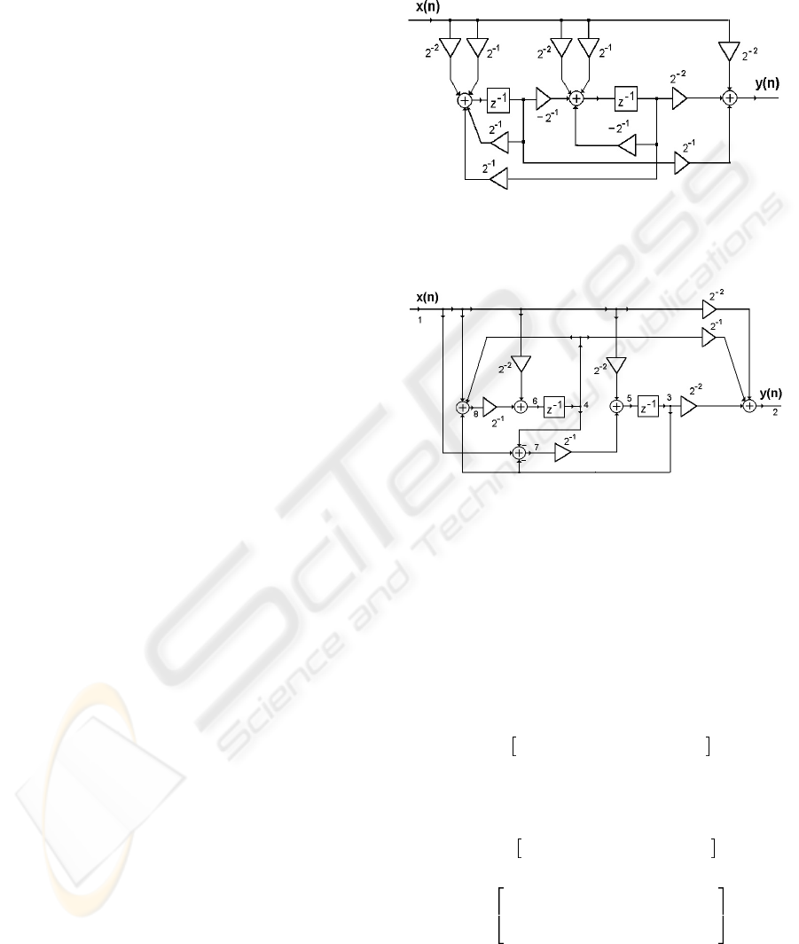
In figure 4 there is a classical structure of the state-
space filter of the second order that has 11 shift oper-
ations. In figure 5 the proposed equivalent state-space
structure of the second order is presented with only
7 shift operations. It can be easily verified that both
structures have the same impulse response.
Figure 4: Classical state-space structure of the second order.
Figure 5: State-space structure without multipliers.
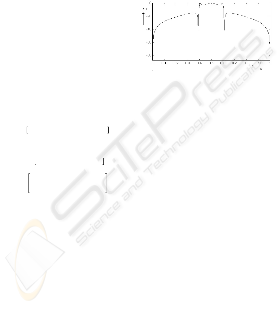
In the second example, we shall calculate the elliptic
low-pass state space filter of the third order, n=3, with
attenuation in the band-pass a
max
=2dB, corner
frequency f
1
=0.6 and attenuation in the band-stop
a
min
=15dB. By means of MATLAB command
[a,b,c,d]= ellip(3,2,15,0.6) we obtain the state-space
matrices for the elliptic low-pass filter with the values:
C =
0.1887 0.0360 0.0680
D =0.3673
B
T
=
2.1724 0.9698 1.3201
A =
0.1160 0.0000 0.0000
0.4982 −0.3513 −0.8830
0.6782 0.8830 −0.2019
With the following equations that realize low-pass
state-space filter of the 3rd order we can obtain the
impulse response yn(i) in the frequency domain. The
ICINCO 2005 - SIGNAL PROCESSING, SYSTEMS MODELING AND CONTROL
26
equations for calculating yn(i), n6, n7, n8 etc. were
derived from figure 3.
a11=0.1160;a12=0.0000;a13=0.0000;
a21=0.4982;a22=-0.3513;a23=-0.8830;
a31=0.6782;a32=0.8830;a33=-0.2019;
b1=2.1724;b2=0.9698;b3=1.3201;
c1=0.1887;c2=0.0360;c3=0.0680;d=0.3673;
n3=0;n4=0;n5=0;
xn=1;
for i=1:1:200
yn(i)=xn
*
d+n3
*
c1+n4
*
c2+n5
*
c3;
n6=xn
*
b1+n3
*
a11+n4
*
a12+n5
*
a13;
n7=xn
*
b2+n3
*
a21+n4
*
a22+n5
*
a23;
n8=xn
*
b3+n3
*
a31+n4
*
a32+n5
*
a33;
n3=n6;n4=n7;n5=n8;xn=0;
end
[h,w]=freqz(yn,1,200);
plot(w,20
*
log10(abs(h)))
In the third example we shall calculate the high-pass
elliptic filter with the specification n=3, a
max
=
2 dB, a
min
=15dB and corner frequency
f
−1
=0.4. By means of MATLAB commands
[a,b,c,d]=ellip(3,2,15,0.4,’high’) we obtain the state-
space matrices for the elliptic high-pass filter in the
form
C =
−0.2597 −0.0495 −0.0936
D =0.3673
B
T
=
1.5783 0.7046 0.9591
A =
−0.1160 0.0000 0.0000
−0.4982 0.3513 0.8830
−0.6782 −0.8830 0.2019
For the analysis of the high-pass filter we have used
the same equation as for the low-pass, but the con-
stants a
ij
, b
i
and c
i
in the program must be changed.
In the fourth example we shall realize the elliptic
band-pass state-space filter for the lower and up-
per corner frequencies 0.4 and 0.6 respectively, and
a
min
=15dB. Using MATLAB commands we get
the state matrices a,b,c and d.
[a,b,c,d]=ellip(3,3,15,[0.4,0.6])
a=
-0.1374 0 0 0.8626 0 0
0.2458 -0.1229 -0.2791 0.2458 0.8771 -0.2791
0.0782 0.2791 -0.0888 0.0782 0.2791 0.9112
-0.8626 0 0 0.1374 0 0
-0.2458 -0.8771 0.2791 -0.2458 0.1229 0.2791
-0.0782 -0.2791 -0.9112 -0.0782 -0.2791 0.0888
b=
0.7927
0.2259
0.0719
-0.7927
-0.2259
-0.0719
c=
0.1125 -0.0022 0.0420 0.1125 -0.0022 0.0420
d=
0.1034
The general structure for the state-space filter of the
arbitrary order can be derived from the structure in
figure 3. To analyze the structure by MATLAB in
the figure 3, the following algorithm must be used.
The attenuation of the band-pass state-space filter is
presented in figure 6.
Figure 6: Attenuation of the band-pass state-space Cauer
Filter.
A11=-0.137;A12=0.000;A13=0.000;A14=0.862;A15=0.000;
A16=0.000;A21=0.245;A22=-0.122;A23=-0.279;A24=0.245;
A25=0.877;A26=-0.279;A31=0.078;A32=0.279;A33=-0.088;
A34=0.078;A35=0.279;A36=0.911;A41=-0.862;A42=0.000;
A43=0.000;A44=0.137;A45=0.000;A46=0.000;A51=-0.245;
A52=-0.877;A53=0.279;A54=-0.245;A55=0.122;A56=0.279;
A61=-0.078;A62=-0.279;A63=-0.911;A64=-0.078;
A65=-0.279;A66=0.088;B1=0.792;B2=0.225;B3=0.071;
B4=-0.792;B5=-0.225;B6=-0.071;C1=0.112;C2=-0.002;
C3=0.042;C4=0.112;C5=-0.002;C6=0.042;D=0.1034;
N3=0;N4=0;N5=0;N6=0;N7=0;N8=0;XN=1;
for i=1:1:500
YN(i)=D
*
XN+N3
*
C1+N4
*
C2+N5
*
C3+N6
*
C4+N7
*
C5+N8
*
C6;
N9 =B1
*
XN+N3
*
A11+N4
*
A12+N5
*
A13+N6
*
A14+N7
*
A15+N8
*
A16;
N10=B2
*
XN+N3
*
A21+N4
*
A22+N5
*
A23+N6
*
A24+N7
*
A25+N8
*
A26;
N11=B3
*
XN+N3
*
A31+N4
*
A32+N5
*
A33+N6
*
A34+N7
*
A35+N8
*
A36;
N12=B4
*
XN+N3
*
A41+N4
*
A42+N5
*
A43+N6
*
A44+N7
*
A45+N8
*
A46;
N13=B5
*
XN+N3
*
A51+N4
*
A52+N5
*
A53+N6
*
A54+N7
*
A55+N8
*
A56;
N14=B6
*
XN+N3
*
A61+N4
*
A62+N5
*
A63+N6
*
A64+N7
*
A65+N8
*
A66;
N3=N9;N4=N10;N5=N11;N6=N12;N7=N13;N8=N14;XN=0;
end
[h,w]=freqz(YN,1,500);
plot(w,20
*
log10(abs(h)))
4.2 Design of the filter from the
transfer function by matrix
method
In this part we shall derive the structure of the digital
filter without multipliers that has the transfer function
(29)
H(z)=
P (z)
Q(z)
=
0.3437 − 0.2890z
−1
+0.4296z
−2
1+0.0625z
−1
− 0.4218z
−2
(29)
ANALYSIS AND SYNTHESIS OF DIGITAL STRUCTURE BY MATRIX METHOD
27
The constants of the transfer function (29) can be de-
composed into the following expression
0.34375 = 2
−2
+2
−4
+2
−5
0.2890 = 2
−2
+2
−5
+2
−7
0.4296 = 2
−2
+2
−3
+2
−5
+2
−6
+2
−7
0.0625 = 2
−4
0.4218 = 2
−2
+2
−3
+2
−5
+2
−6
First of all the matrix N
(3)
in the form (30) must be
written
N
(3)
=
0 −11
P (z)0−Q(z)
(30)
N
(3)
=
⎡
⎢
⎢
⎢
⎣
0 −1 1
2
−2
+2
−4
+2
−5
0 −1 − z
−1
2
−4
−z
−1
(2
−2
+2
−5
+2
−7
) +z
−2
(2
−2
+2
−3
+z
−2
(2
−2
+2
−3
+ +2
−5
+2
−6
)
2
−5
+2
−6
+2
−7
)
⎤
⎥
⎥
⎥
⎦
(31)
In this case we shall expand transfer matrix N
(3)
equation (31), so the signal U
i
must be added. If we
choose in the matrix N
(4)
the element n
(4)
24
=0the
elements in the first row remain unchanged. In case
that n
(4)
34
=2
−5
and n
(4)
41
=1−z
−1
−z
−2
are chosen
then element n
(4)
31
in the matrix N
(4)
acquire the value
2
−2
+2
−4
− z
−1
(2
−2
+2
−7
)+z
−2
(2
−2
+2
−3
+
2
−6
+2
−7
). Similarly if the element n
(4)
43
= z
−2
will
be chosen then the element n
(4)
33
in the matrix N
(4)
ac-
quire the value −1−z
−1
2
−4
+z
−2
(2
−2
+2
−3
+2
−6
).
The element n
(4)
44
must be equal -1.
N
(4)
=
⎡
⎢
⎢
⎢
⎢
⎣
0 −1 1 0
2
−2
+2
−4
− 0 −1 − z
−1
2
−4
+ 2
−5
z
−1
(2
−2
+2
−7
) z
−2
(2
−2
+2
−3
+2
−6
)
+z
−2
(2
−2
+2
−3
+2
−6
+2
−7
)
1 − z
−1
+ z
−2
0 z
−2
−1
⎤
⎥
⎥
⎥
⎥
⎦
(32)
In the new matrix N
(5)
the elements in the last row
and last column can be chosen. Provided that we
choose elements n
(5)
ij
in the matrix N
(5)
in this way
n
(5)
25
=0, n
(5)
35
=2
−2
, n
(5)
45
=0, n
(5)
55
= −1, we ob-
tain n
(5)
51
=1− z
−1
+ z
−2
, n
(5)
52
=0, n
(5)
53
= z
−2
and n
(5)
54
=0and we get the equation (33) from the
equation (32).
N
(5)
=
⎡
⎢
⎢
⎢
⎢
⎣
0 −1 1 0 0
2
−4
− z
−1
(2
−7
) 0 −1 − z
−1
2
−4
2
−5
2
−2
+z
−2
(2
−3
+2
−6
+z
−2
(2
−3
+2
−6
)
+2
−7
)
1 − z
−1
+ z
−2
0 z
−2
−1 0
1 − z
−1
+ z
−2
0 z
−2
0 −1
⎤
⎥
⎥
⎥
⎥
⎦
(33)
In the new matrix N
(6)
the elements in the last row
and last column can be chosen again. In case that
we choose elements n
(6)
ij
in the matrix N
(6)
in this
manner n
(6)
26
=0, n
(6)
36
=2
−3
, n
(6)
46
=0, n
(6)
56
=0,
n
(6)
66
= −1, we get n
(6)
61
= z
−2
, n
(6)
62
=0, n
(6)
63
=
z
−2
, n
(6)
64
=0, n
(6)
65
=0and we obtain the equation
(34) from the equation (33).
N
(6)
=
⎡
⎢
⎢
⎢
⎢
⎢
⎣
0 −1 1 0 0 0
2
−4
− z
−1
2
−7
0 −1 − z
−1
2
−4
2
−5
2
−2
2
−3
+z
−2
(2
−6
+2
−7
) +z
−2
2
−6
1 − z
−1
+ z
−2
0 z
−2
−1 0 0
1 − z
−1
+ z
−2
0 z
−2
0 −1 0
z
−2
0 z
−2
0 0 −1
⎤
⎥
⎥
⎥
⎥
⎥
⎦
(34)
In case that we choose elements n
(7)
ij
in the matrix
N
(7)
in this manner n
(7)
27
=0, n
(7)
37
=2
−6
, n
(7)
47
=0,
n
(7)
57
=0, n
(7)
67
=0, n
(7)
77
= −1, we get n
(7)
71
= z
−2
,
n
(7)
72
=0, n
(7)
73
= z
−2
, n
(7)
74
=0, n
(7)
75
=0, n
(7)
76
=
0 and we obtain the equation (35) from the equation
(34).
N
(7)
=
⎡
⎢
⎢
⎢
⎢
⎢
⎢
⎢
⎢
⎢
⎢
⎣
0 −1 1 0 0 0 0
2
−4
− z
−1
2
−7
0 −1 − z
−1
2
−4
2
−5
2
−2
2
−3
2
−6
+z
−2
2
−7
1 − z
−1
0 z
−2
−1 0 0 0
+z
−2
1 − z
−1
0 z
−2
0 −1 0 0
+z
−2
z
−2
0 z
−2
0 0 −1 0
z
−2
0 z
−2
0 0 0 −1
⎤
⎥
⎥
⎥
⎥
⎥
⎥
⎥
⎥
⎥
⎥
⎦
(35)
Following with this procedure we obtain the matrix
N
(14)
s
. The matrix N
(14)
s
is the signal-flow matrix
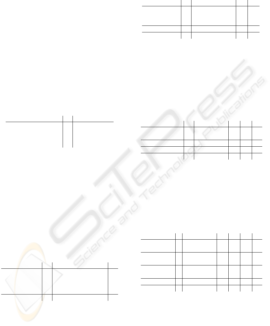
and from this matrix the circuit can be drawn. The
structure that correspond to the signal-flow matrix
(36) is presented in the figure 7 with minimum shift
operations. In the figure 8 A) is shown the equivalent
filter with 16 shift operations and the figure 8 B) dis-
plays the filter with 5 multipliers. The circuits in the
figure 7 and 8 have the same impulse response.
ICINCO 2005 - SIGNAL PROCESSING, SYSTEMS MODELING AND CONTROL
28
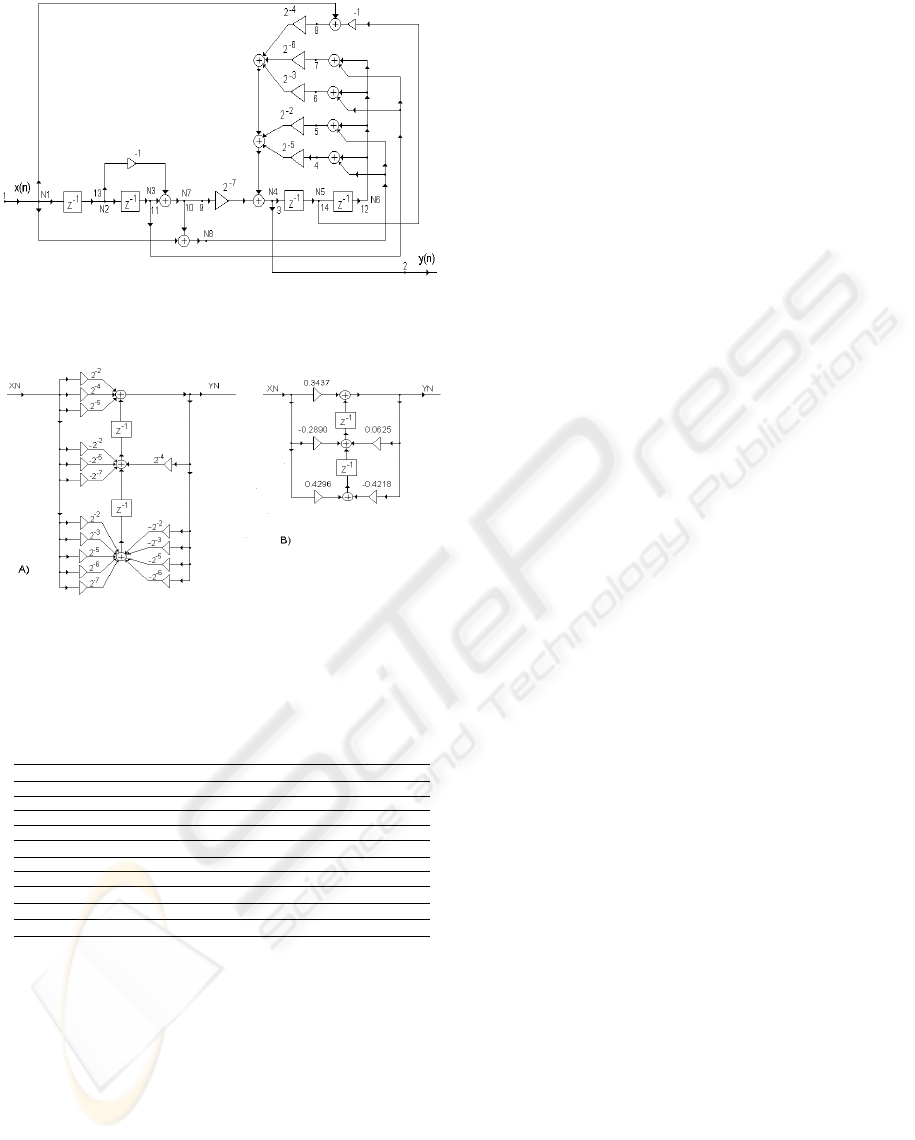
Figure 7: Digital filter with 6 shift operation.
Figure 8: Classical circuit of the digital filter A) with shift
operation B) with multiplication.
N
(14)
s
=
⎡
⎢
⎢
⎢
⎢
⎢
⎢
⎢
⎢
⎢
⎢
⎢
⎣
0 −1100000000000
00−12
−5
2
−2
2
−3
2
−6
2
−4
2
−7
000 0 0
10 0 −10000010100
10 0 0 −1000010100
00 0 0 0 −100001100
000000−10 001100
10z
−1
0000−100000−1
00000000−1100 0 0
000000000−11 0 −10
0000000000−10z
−1
0
00000000000−10z
−1
z
−1
00000000000−10
00z
−1
0000000000−1
⎤
⎥
⎥
⎥
⎥
⎥
⎥
⎥
⎥
⎥
⎥
⎥
⎦
(36)
5 CONCLUSION
The method proposed in this paper allows the analysis
of digital networks and the construction of new state
digital filters. Equivalent filters of differing structures
can be found according to various matrix expansion.
By this procedure structures can also be obtained
without multipliers. This matrix method synthesis of
the digital structures seems to be laborious, but in fact
it is very simple and the effects are satisfactory when
are evaluated using the analysis of the structures. The
parts of the MATLAB programs can be used for im-
plantation of the low-pass, high-pass and band-pass
state-space filter in digital signal processor DSP.
REFERENCES
R. Luecker, Matrixbeschreibung und Analyse zeit discreter
Systeme., Forschungsbericht Nr. 81. Informationsbib-
liothek Hannover: RN 2251. 1976.
B. P
ˇ
seni
ˇ
cka and G. Herrera, Synthesis of Digital Filters by
Matrix Method. Proceedings of the IASTED Interna-
tional Conference on Signal and Image Processing.
SIP 97. December 4-6, 1997, New Orleans, Louisiana,
USA. pp.409-412.
B. P
ˇ
seni
ˇ
cka and F. Garc
´
ıa Ugalde, Design of State Digi-
tal Filters without Multipliers. ICSPAT 7-19 October
1999, USA.
B. Psenicka, F. Ugalde and J. Savage, Design of State Digi-
tal Filters. IEEE Trans. on Signal Processing. Volume
46, Number 9, pp. 2544-2549, September 1998.
C. W. Barnes, On the Design of Optimal State-Space Real-
izations of Second-Order Digital Filters. IEEE Trans.
on CAS, Vol. 31, No. 7, pp. 602–608, July 1984.
B.W. Bomar, New Second-Order State-Space Structures for
Realizing Low Roundoff Noise Digital Filters. IEEE
Trans. on ASSP, Vol. 33, No. 1, pp. 106–110, February
1985.
B.W. Bomar, Computationally Efficient Low Roundoff
Noise Second-Order State-Space Structures. IEEE
Trans. on CAS, Vol. 33, No. 1, pp. 35–41, January
1986.
Z. Sm
´
ekal and R. V
´
ıch R, Optimized Models of IIR Digital
Filters for Fixed Point Digital Signal Processor. Pro-
ceedings of the 6th IEEE International Conference on
Electronics Circuits and System ICES 99. September
5-8 1999, Cyprus, pp 145-148. ISBN 0-7803-5682-9.
Z. Sm
´
ekal, Spectral Analysis and Digital Filter Banks. Pro-
ceedings of the International Conference on Research
in Telecommunication Technology. (RTT 2001), Sep-
tember 24-26, 2001, Lednice, Czech Republik, pp. 67-
70. ISBN 80-214-1938-5.
ANALYSIS AND SYNTHESIS OF DIGITAL STRUCTURE BY MATRIX METHOD
29
