
INFORMATION-BASED INVERSE KINEMATCS MODELING
FOR ANIMATION AND ROBOTICS
Mikyung Kim and Mahmoud Tarokh
Department of Computer Science. San Diego State University, San Diego, CA 92124, U.S.A.
Keywords: Inverse kinematics, robotics, Neural networks, Animation.
Abstract: The paper proposes a novel method for extremely fast inverse kinematics computation suitable for
animation of anthropomorphic limbs, and fast moving lightweight manipulators. In the information
intensive preprocessing phase, the workspace of the robot is decomposed into small cells, and joint angle
vectors (configurations) and end-effector position/ orientation (posture) data sets are generated randomly in
each cell using the forward kinematics. Due to the existence of multiple solutions for a desired posture, the
generated configurations form clusters in the joint space which are classified. After the classification, the
data belonging to each solution is used to determine the parameters of simple polynomial or neural network
models that closely approximates the inverse kinematics within a cell. These parameters are stored in a
lookup file. During the online phase, given the desired posture, the index of the appropriate cell is found,
the model parameters are retrieved, and the joint angles are computed. The advantages of the proposed
method over the existing approaches are discussed in the paper. In particular, the method is complete
(provides all solutions), and is extremely fast. Statistical analyses for an industrial manipulator and an
anthropomorphic arm are provided using both polynomial and neural network inverse kinematics models,
which demonstrate the performance of the proposed method.
1 INTRODUCTION
One of the most fundamental and ever present
problems in computer animation and robotics is the
inverse kinematics (IK). This problem maybe posed
as follows: Given a desired posture vector u
representing the hand (end-effector) position and
orientation, and the forward kinematics equation
)(fu
θ
= , find the set of all joint angle vectors
(configurations)
θ
of the animation character or
manipulator that satisfy the forward kinematics
equation. The IK mapping is in general one to
many, involves complex inverse trigonometric
functions, and for most manipulators and animation
figures no closed form solution exists. In addition, in
computer animation, as well as in real-time
manipulator applications, extremely fast IK
computation is required.
The IK problem has attracted immense attention
and numerous solutions have been proposed,
including algebraic, Jacobian-based and
neural/genetic algorithms. In the algebraic based
approaches, a system of nonlinear polynomial
equations in the elements of
θ
is solved either
symbolically or numerically using various methods
(Uicker 1984, Manchoa 1994, Zhao 1994, Tolani
2000). Algebraic methods are generally
computationally intensive and are not suitable for
applications such as animation that require
extremely fast solutions.
Jacobian based approaches (e.g. Whitney 1972,
Press 1988), formulate problem at the velocity
level, i.e.
)t()(J)t(u
θθ
=
where J(q) is the
Jacobian matrix of the manipulator. The equation is
solved for the joint rate vector
)t(
θ
, which is then
integrated to obtain
θ
. When the manipulator is
redundant, the Jacobian matrix becomes non-square,
and several approaches such as Jacobian pseudo-
inverse and Jacobian augmentation have been
proposed to resolve the redundancy (e.g. Klein
1983, Seraji 1993). One of the main difficulties with
the Jacobian based approaches is the singularity
problem where J(q) becomes rank deficient, which
can cause joint velocities (and acceleration/jerk) to
become unacceptably large. To ameliorate the
singularity problem, a number of methods have been
proposed (e.g. Chiacchio 1991, Chiaverini 1994,
76
Kim M. and Tarokh M. (2005).
INFORMATION-BASED INVERSE KINEMATCS MODELING FOR ANIMATION AND ROBOTICS.
In Proceedings of the Second International Conference on Informatics in Control, Automation and Robotics - Robotics and Automation, pages 76-84
DOI: 10.5220/0001164600760084
Copyright
c
SciTePress

Lloyd 2001), each requiring special considerations
to deal with singularities with the associated
computation overhead. More importantly, they are
not complete in the sense that they do not provide all
solutions (configurations) for a given posture.
More recently, neural networks and genetic
algorithms have been used for solving the inverse
kinematics problem (e.g. Dermata 1996, Nearchou
1998, Khwaja 1998, Chapelle 2001, De Lope 2003).
Neural network and genetic algorithm methods are
not complete and therefore generally find a
particular solution rather than all solutions. Neural
networks face problems for approximating multi-
valued functions. Genetic algorithms do not
guarantee the convergence to a desired solution, but
their major difficulty is that they require many
generations (iterations) to arrive at an approximate
solution and therefore are not suitable for real-time
applications.
The purpose of this paper is to propose a novel
approach for ultra fast IK solutions with few
limitations for 6-DOF manipulators, and 7-DOF
anthropomorphic limbs used in animation. Fast IK
techniques are needed for multiple limb animation
characters such as a human figure for variety of
applications such as motion capture. The IK
problem is solved in two phases, an off-line
information-based preprocessing phase and an on-
line rapid evaluation phase. Preprocessing consists
of spatial decomposition, classification, optimal data
generation and simple polynomial curve fitting, or
neural network approximation. This off-line
preprocessing phase is performed only once for a
limb or a manipulator, and can be used an infinite
number of times during on-line IK computation.
Because of the preprocessing, the on-line phase,
which finds various configurations for a desired
posture, is extremely fast.
2 SPATIAL DECOMPOSITION
In this section we discuss the forward kinematics
and spatial decomposition for 7-DOF limbs and
manipulators. All the developments of this and
subsequent section will naturally be valid for the
cases with fewer 7-DOF, as will be demonstrated in
Section 5.
A human-like figure, often used in animation
and graphics, consists of a number of limbs i.e. arms
and legs. An arm (leg) is generally modeled as a 7
DOF chain consisting of the shoulder (hip) and the
wrist (ankle) each as a 3 DOF spherical joint, and
the elbow (knee) as a single DOF revolute joint
(Tolani 2000). The human-like figure is often
decomposed into limbs with the torso as the
common or reference coordinate. In motion capture
applications, position and orientation of the shoulder
(hip) and hand (foot) of a live subject are measured
using sensors attached to the body. The position and
orientation are then used in conjunction with inverse
kinematics to find the joint angles of the limbs in
order to drive animation characters. It is also noted
that most redundant robot manipulators used in
applications or in research are also 7 DOF (Seraji
1993). Examples of these manipulators are the
space station RMS and K1207 manufactured by
Robotics Research arm. The latter has a joint and
links arrangements similar to limb, but it also has
offset at joints.
Consider the forward kinematics equation of a
limb
)(fu
θ
=
(1)
where
θ
is the 17
×
vector of joint angles that define
the limb configuration, and u is the
16 × vector of
the limb posture which defines the hand position
(e.g. x, y, z) and orientation (e.g. Euler angles
γ
β
α
,, ). We refer to the 7-dimensional space
whose the coordinates are the joint angles as the
configuration space and to the 6-dimensional space
whose coordinates are position and orientation as the
posture space. Because the dimension of the
configuration space is more than that of posture
space, the anthropomorphic limb has redundancy.
In order to encode and exploit the redundancy,
we parameterize the solution space using a single
variable v. This variable is specified on-line to
explore different solutions and choose the one best
suited for the application on hand. Elbow
inclination in a 7-DOF anthropomorphic limb or in
the K1207 manipulator is an example of such a
variable. The elbow inclination is defined as the
angle of the rotation, about the shoulder-wrist line,
of the plane containing origins of shoulder, elbow
and wrist. The elbow inclination, referred to as
swivel angle in (Tolani 2000) and as arm angle in
(Seraji 1993), has been used to constrain a selected
point on the limb, to perform aiming of the end-
effector towards a target point, to keep the figure
balanced, etc. (Tolani 2000)
The elbow inclination v can be written as
)(gv
θ
=
(2)
INFORMATION-BASED INVERSE KINEMATCS MODELING FOR ANIMATION AND ROBOTICS
77

where
)(g
θ
is a kinematics function that relates the
joint angles to the elbow inclination mentioned. In
the limb, v is in fact a function of only the first four
joint angles. We now augment kinematics equation
(1) with the variable constraint equation (2) to
obtain
⎟
⎟
⎠
⎞
⎜
⎜
⎝
⎛
=
⎟
⎟
⎠
⎞
⎜
⎜
⎝
⎛
)(g
)(f
v
u
θ
θ
or )(hw
θ
= (3)
The new posture is now the
17 × vector
T
)vu(w = , the forward kinematics function is
T
))(g)(f()(h
θθθ
= and (3) represents the
kinematics of a non-redundant limb. The result of
the kinematics constraint is an increase in the
dimension of the posture space from 6 to 7.
We now decompose the posture space into
small cells so that the IK can be approximated by
very simple expression in each cell. These 7-
dimensional cells have their axes representing
positions
z
,y,
x
, orientation angles
γ
βα ,, (using a
suitable convention such as Euler angles), and v (e.g.
elbow inclination). The cell side lengths are
obtained by dividing the maximum ranges of each
quantity,
γ
β
α
,,,v,z,y,x into a number of
divisions
γ
N,,N,N
yx
"
. Any valid limb posture
will be in one of the cells defined above. Higher
values of
γ
N,,N,N
yx
"
correspond to smaller size
(volume) cells and result in more cells, adding to the
off-line computation effort. However, smaller cell
sizes will require simpler mathematical models for
representing the cell inverse kinematics. These
simpler models in turn speed up the on-line
computation effort.
Once the posture space is decomposed into the
cells, we must generate data points for each cell. The
data consists of sets of configuration vectors
θ
and
their associated postures vectors w. A large number
of configurations are generated by assigning random
values in the range of joints angles, and (3) is used
to determine their respective posture w. Each
generated posture is placed into its appropriate cell,
and when the number of postures in a cell reaches a
predetermined value
p
N , the next generated
posture that falls into that cell is discarded. The
generation continues until a certain percentage of the
cells have
p
N
postures. It is noted that many cells
may be outside the workspace in which case they
will not contain any postures, and some cells are on
the boundary or partially in the workspace in which
case they will contain fewer than
p
N
postures.
3 CLASSIFICATION
The generated cell configuration-posture data set
}w,{
θ
cannot be used for modelling without further
processing. First, it is noted that there can be a
number of configurations (solutions) for a given
posture. The anthropomorphic limb has a spherical 3
DOF shoulder joint (
321
,,
θ
θ
θ
) which together with
the a single DOF elbow joint (
4
θ
) can achieve a
desired wrist position/elbow inclination (sub-
posture) with a maximum of four sets of joint
angles (sub-configurations), namely,
(
4321
,,,
θ
θ
θ
θ
), (
4321
,,,
θ
π
θ
θ
θ
+ ),
(
4321
θ
θ
π
θ
π
θ
,,,
−
−
+
) and
(
4321
θ
π
θ
π
θ
π
θ
,,,
+
−
−
+
). It is noted that only
the first three angles are responsible for providing
different solution. In addition, the wrist is also a
spherical joint, and a desired hand orientation can be
achieved with two sets of wrist joint angles
765
,,
θ
θ
θ
. Thus the maximum number of solutions
(configurations) for a desired posture is eight. The
kinematics of the limb is such that the hand position
and elbow inclination
v,
z
,y,
x
are dependent only
on the first four joint angles
41
θ
θ
,," . The wrist
angles
765
θ
θ
θ
,, are dependent both on these four
joints and the desired orientation
γ
β
α
,, .
Before cell IK modelling, configuration-posture
data belonging to a solution must be separated from
those of the other solutions within a cell. In (Tarokh
2005), we have developed a fuzzy classification
method to classify the solutions.
4 INVERSE KINEMATICS
MODELING
The purpose of this step in the preprocessing phase
is to develop a simple model for the IK, and to
determine its parameters for each solution within
each cell. The simplicity or complexity of the
required model depends on the size of the cell.
Smaller size cells will require simpler models to
accurately represent postures in them, but the
number of cells will be higher since the posture
space volume is constant. The opposite is true for
larger cell sizes, which require more complex
ICINCO 2005 - ROBOTICS AND AUTOMATION
78

models. For animation, high position/orientation
accuracy is not essential, but very short online
computation time is needed, and therefore a simple
model is preferred. We consider two models,
namely polynomial and neural network models as
follows:
4.1 Polynomial Model
The simplest polynomial model representing the
relationship between the first four joint angles and
position/inclination belonging to a particular
solution in a cell is the linear equation
T
ii i
a(xyzv) i 1,2, ,4
θσ
=+="
(4)
where
i
a is a 41× constant parameter vector and
i
σ is a constant scalar parameter. These parameters
are determined via a least squares (regression)
method for each cell using the cell data set. Note
that the same accuracy of the inverse kinematics
solution can be obtained by reducing the number of
cells but increasing the order of the model which in
turn increases the number of model parameters and
online computation time.
The model parameters are stored as records in a file
for the subsequent online retrieval. Each record has a
unique address in the file where the parameters of a
cell inverse kinematics model are stored. Suppose
there are D divisions for each of the axes
v,
z
,y,
x
.
Then there will be
4
cell
DD= cells, and the file
address is encoded as
32
adrs 4 3 2 1
F
kD kD kD k=+++ (5)
where
14
k,,k " are integers between 0 and D1
−
,
and represent the cell indices for
v,
z
,y,
x
. At each
address representing a cell, there is a solution
number, followed by the values of model parameters
(
ii
,a
σ
) for the particular cell and solution.
During the online phase, given the desired sub-
posture (e.g.
dddd
v,z,y,x ), the cell indices
134
k,,k,k " are computed as follows. Suppose the
range of a posture variable, say v, is
min
v to
max
v ,
and the cell size length is
s
l
v , then the index
1
k is
computed as
dmin
1
sl
vv
k ceil
v
⎛⎞
−
=
⎜⎟
⎝⎠
(6)
where ceil denotes the ceiling of the quantity. Other
cell indices
432
k,k,kfor
x
,y,zare computed
similarly and the address in the file is determined via
(5).
Since the data is stored in the file with
increasing order of the address, a binary search is
conducted to locate and access the cell data. The
binary search performs
)N(log
cell2
comparisons in
the worst case. Once the parameters for each
solution are retrieved, the joint angle values are
computed via (4).
The wrist joint angles
765
θ
θ
θ
,, are modeled
similarly to achieve the desired orientation.
However, these joints angle are dependent both on
the first four joints and the desired orientation. In
addition the wrist joint angles have a more complex
relationship with the orientation. As a result we
express the wrist angles as a linear relation with the
first four joint angles and a quadratic relation with
the orientation angles of the form
TT
ii1234 i
T222
iii
b( ) c( )
d( ) e( )
i5,6,7
θθθθθ αβγ
α
βαγ βγ α β γ σ
=+
+
++
=
(7)
where
i
b is a 41
×
parameter vector,
i
c ,
i
d and
i
e
are
31
×
parameter vectors and
i
σ is a scalar
parameter. These parameters are obtained using a
least squares method, and are stored as records
similar to the procedure given above for the first
four joint angles. The cells for the orientation will
be 7-dimensional, and (5) will be a 6-th order
polynomial. The on-line procedure is also identical
to those of first four joint angles. Since no
trigonometric or inverse trigonometric functions are
involved, the computation is extremely fast.
4.2 Neural Network Model
It is well known that backpropagation neural
networks can be used for approximation. In this
section we describe a simple neural network model
to approximate the inverse kinematics relationship.
For the position kinematics, the neural network
consists of an input layer with a
4N× weight
matrix
in
W , where 4 is the number of inputs
INFORMATION-BASED INVERSE KINEMATCS MODELING FOR ANIMATION AND ROBOTICS
79
v,
z
,y,
x
, N is number of neurons in the hidden
layer, and the output layer has 4 outputs representing
4321
,,,
θ
θ
θ
θ
. The inputs v,
z
,y,
x
are first
normalized as
min
max min
2( x x )
x
1
(x x )
−
=−
−
(8)
where
min
x
and
max
x
are, respectively the minimum
and maximum values of the x data in the cell.
Similarly
y,z,v are normalized so that their ranges
are between –1 and +1. The output of the input
layer p is thus
in in
ˆˆ ˆ
ˆ
p(xyzv)W b=+
(9)
where
in
b is a constant 1N× bias vector. A
tangent sigmoid function of the following form is
applied to p to obtain
j
j
2p
2
q 1; j 1,2,...N
1e
−
=−=
+
(10)
Finally, the normalized joint angle vector is obtained
from
1234 outout
ˆˆˆˆ
()qWb
θθθθ
=+ (11)
where q is an
1N× vector
out
W is an N4× matrix
and
out
b is a 14× output bias. The actual
(denormalized) joint angles are obtained from
i i,max i,min i i,min
1
ˆ
()(1)
2
θθθθ θ
=− ++ (12)
where
i,max i,min
,
θ
θ
are the minimum and maximum
values of
i
θ
in the cell. The neural network is then
trained with the cell data points to obtain weight
matrices and bias vectors.
The data to be stored for the on-line phase are the
weight matrices
in
W and
out
W , bias vectors
in
b and
out
b and minimum and maximum of
v,
z
,y,
x
,
12 34
,,,
θ
θθθ
for each cell. During the on-
line phase, given the desired values of
v,
z
,y,
x
,
these values are normalized via (8), passed through
the input, hidden and output layers by applying (9)-
(11). The actual (denormalized) joints values are
finally found from (12).
Orientation kinematics is obtained similarly to
the above, except that the inputs to the network
are
12 34
,,,
θ
θθθ
obtained above and the orientation
angles
γ
β
α
,, . The outputs of the network are the
joint angles
567
,,
θ
θθ
. The input and output
weight matrices
in
W and
out
W are now 7N× and
N3
×
, and the bias vectors
in
b and
out
b are
1N
×
and 13
×
, respectively.
5 PERFORMANCE ANALYSIS
In this section we apply the proposed method to the
Puma 560 manipulator and the anthropomorphic
arm. The reason for the choice of the Puma 560 is
that it is a well known and extensively researched
manipulator, and serves as a bench mark.
Furthermore, it has a closed form inverse kinematics
and thus the correctness and success rate of the
proposed method can be checked against the known
results of the Puma 560.
5.1 IK Modeling of Puma 560
The joint angles ranges of the Puma are given in
Table 1. The first three joints, or the major joints, of
the Puma 560 are waist, shoulder and elbow joints,
and determine the position of the end-effector.
Therefore, we can express the first three joints in
terms of
x, y and z only. The fully stretched arm is
about
900 mm long, and we assign ranges for each of
x, y and z directions from –900 mm to +900 mm,
with the cell side length of 200 mm which forms
cubes of volume
3
100 100 100 mm×× . There are a
maximum of
(
)
3
1800
100
5832= cubes (cells), but only
about 3400 of them contained generated postures
due to the joint angle limits. The maximum number
of cells for the orientation kinematics with cells
sizes of 20 degrees for
12 3
,,
θ
θθ
, and 45 degrees for
γ
β
α
,, for the ranges of these angles are
17 14 17 8 8 8 2,071,552
×
××××= .
We used the polynomial model (4) and (7).
The number of joints for position is three and only x,
y and z are present, thus
i
a , i=1,2,3 in (4) are
31
×
vectors.
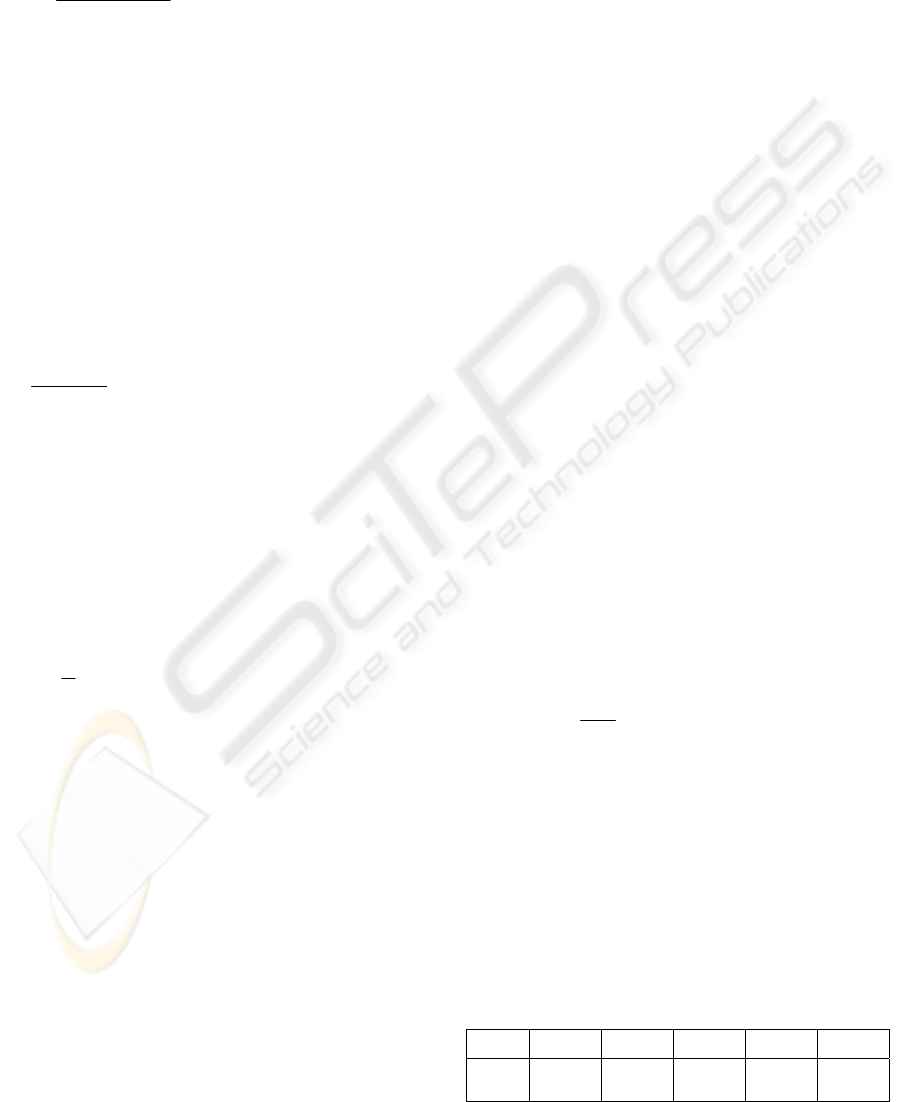
Table 1: Joint angle ranges (limits) for Puma 560
1
θ
2
θ
3
θ
4
θ
5
θ
6
θ
–170
+170
–225
+45
–250
+75
–135
+135
–100
+100
–180
+180
ICINCO 2005 - ROBOTICS AND AUTOMATION
80
The Puma 560 has a maximum of four
solutions, i.e. elbow up/down, left/right arm, for
positioning of the end-effector, and eight solutions
for position and orientation, which were found using
the classification. The parameters of the above
models were found for each of the four solutions in
each of the cells using a least squares method.
These parameters were stored in a file for each cell,
and the total storage needed was about 372 KB for
position kinematics and 340 MB for the orientation
kinematics. Note that memory and disks are very
cheap (e.g. about $100 per 1 GB of memory and
about $60 for a 100 GB disk), and are readily
available on a PC.
In order to test the validity of the models, we
generated randomly 1000 position and orientation
postures within the ranges of
x, y, z and
γ
β
α
,, .
The polynomial model (4) and (7) were used to
obtain the joint angles. The results are summarized
in Table 2a and Table 2b.
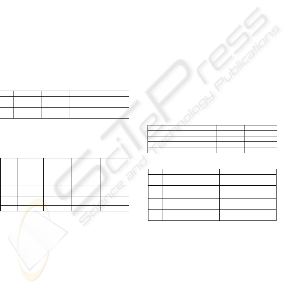
Table 2a: Position kinematics – Polynomial model
A B C D E
1 908 99.3 2.92 2.37
2 500 98.6 2.80 2.17
3 518 98.6 2.83 2.36
4 927 99.2 2.92 2.41
A: Number of solutions
B: Number of valid configurations
C: Success rate (%)
D: Mean absolute position error (mm)
E: Error standard deviation (mm)
Table 2b: Orientation kinematics – Polynomial model
A B C D E
1 340 97.3 2.10 2.92
2 144 97.3 1.96 2.45
3 276 96.2 1.83 2.15
4 372 97.4 1.96 2.34
5 385 98.2 2.22 2.73
6 238 96.0 1.94 2.62
7
196 97.1 1.95 2.88
8 369 95.7 1.81 2.38
A, B , C: as defined in Table 2a.
D: Mean absolute orientation error (degrees)
E: Error standard deviation (degrees)
The success rate is defined as the ratio of the
number of valid configurations found by the method
to those found by the closed-form inverse kinematic
equation. It is seen that the success rates are high
ranging from
89% to 100%. The error is defined as
the difference between the desired and actual end-
effector position, and orientation. The actual values
are determined by substituting the joint angles found
by the method in the forward kinematics equations.
It is seen from Table 2 that the mean absolute
position and orientation errors are about 1.8 mm,
and 4.5 degrees, respectively.
Now consider the neural network model (8)-
(12) applied to the Puma 560, however the cell size
for position was increased to 200 mm providing
only 646 cells for position. The size of orientation
cells is the same as in the case of polynomial model.
Several experiments were conducted to determine
the number of neurons for accuracy, simplicity and
success rate and it was found that
N = 5 provided a compromise among these
characteristics. The maximum amount of memory
needed for storing weight matrices, bias vectors and
minimum and maximum values for normalization
and denormalization were 573 KB for position and
605 MB for orientation which are between 1.5 to 1.7
times of those of the polynomial model.
The results are now summarized in Tables 3a
and 3b. It is seen that the success rates are very high
ranging from 92% to 100%, which are higher than
the polynomial model. The position errors are about
2.5 mm and the orientation errors are 2.9 degrees
which are somewhat better than the polynomial
model given in Table 2. The online time, however,
is two to three times more than the polynomial
model. This is due to the higher number of
parameters and operations needed in the neural
network model.
Table 3a: Position kinematics – neural network model
A B C D E
1 880 91.6 1.74 1.31
2 465 89.1 1.91 1.32
3 451 91.1 1.92 1.42
4 830 94.0 1.77 1.36
A,B,C,D,E : See definitions in Table 2a
Table 3b: Orientation kinematics - neural network model
A B C D E
1 350 97.3 1.75 2.68
2 160 97.3 2.67 2.54
3 260 96.2 3.09 5.62
4 813 97.4 2.33 3.71
5 392 98.2 3.62 6.35
6 205 96.0 2.27 2.94
7 196 97.1 4.41 7.11
8 368 95.7 1.48 1.89
A,B,C,D,E: See definitions in Table 2b.
The total on-line time T to compute different
configurations for a desired posture consists of
several components as follows:
1
T : Checking to verify that the desired point
ddd
z,y,x is reachable.
2
T : Computing the cell indices and the addresses
in the file for position and orientation.
3
T : Applying a binary search to locate the address
in the file where model parameters for various
INFORMATION-BASED INVERSE KINEMATCS MODELING FOR ANIMATION AND ROBOTICS
81
solutions are stored, and retrieving these
parameters.
4
T : Computing joint angles using (4) and (7) for
polynomial model, and (8)-(12) for the neural
network model.
The total computation time is the sum of the above
four time components. The online computation was
done on a Pentium 4, 3.0
GHz computer with a C
program. Table 4 show the total online time for
each model. Note that the time is in microseconds
for computing all solutions (a maximum of eight)
averaged for 1000 randomly generated postures.
For the sake of comparison, the solutions were also
computed using the closed-form inverse kinematics
of the Puma 560. These closed form equations were
programmed in C with an optimized implementation
to perform the least amount of computation. The
total time using the closed-form inverse kinematics
computation was 24 microseconds, which is 10
times slower than the proposed method with the
polynomial model, and 4 times slower than the
neural network model. The contrast is much greater
for robots that do not have closed-form solutions.
Our analysis and simulations have shown that the
proposed method can be two to three orders of
magnitude faster than other techniques for
manipulators without closed forms kinematics.
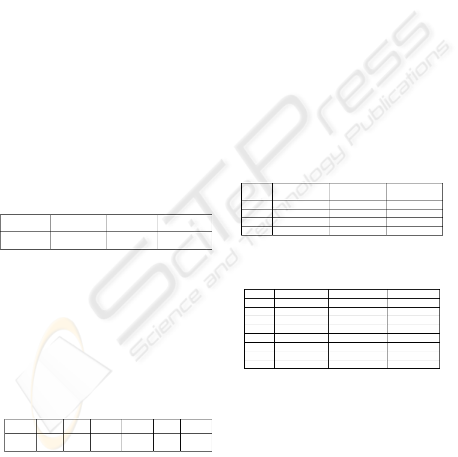
Table 4: Total computation times in microsecond
Polynomial
Position
Polynomial
Orientation
Neural Net
Position
Neural Net
Orientation
0.54
1.58
2.16
4.66
5.2 Modeling of Anthropomorphic
Arm
The procedures described above were applied to the
anthropomorphic arm described before. The ranges
of the spherical shoulder joints (
321
θ
θ
θ
,, ), elbow
(
4
θ
) and the spherical wrist joints (
765
θ
θ
θ
,, ) are
given in Table 5. The upper arm length is 334 mm
and lower arm length is 288 mm. The length and
joint limit data were obtained from a study
conducted by NASA.
Table 5: Joints ranges for the anthropomorphic arm
1
θ
2
θ
3
θ
4
θ
5
θ
6
θ
7
θ
–39
164
–61
187
–83
210
0
149
–40
61
–59
78
–78
94
The fully stretched arm is about 600 mm long,
and we assign ranges for each of
x, y and z from –
600 mm
to +600 mm, with the cell side length of 60
mm
. The range of inclination angle is –100 degrees
to +40 degrees with the cell size of 10 degrees.
With these ranges, the maximum number of cells is
129,654.
The polynomial model (4) for the position
requires a maximum storage of 14.9 MB if all cells
contain data and each cell has the maximum of four
solutions. An experiment involving 1000 randomly
chosen values of (
v,
z
,y,
x
) was carried out and the
values of (
4321
θ
θ
θ
θ
,,, ) were found using the
acquired IK model parameters. These values were
then substituted in the forward kinematics to
determine the accuracy of the solution. Table 6a
shows the number of cells containing 1, 2, 3 or 4
solutions, and the average and standard deviation
position errors for each solution. These errors are
quite acceptable for animation applications.
Furthermore since there is no closed form solution,
the success rate cannot be estimated for the arm, but
is believed to be similar to that of the Puma 560.
Note also that the smaller number of valid solutions
compared to the Puma 560 is due to the limited
ranges of the anthropomorphic arm joint angles and
specification of (restriction on) the elbow
inclination.
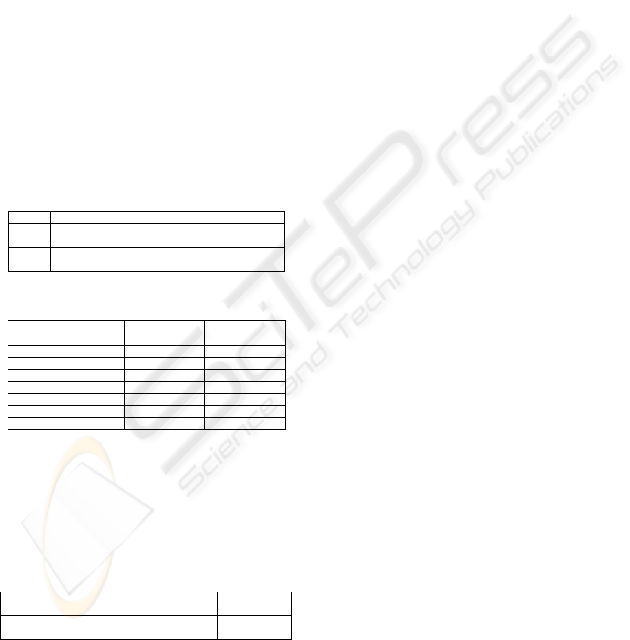
Table 6a: Position kinematics – Polynomial model
A B C D
1 481 1.97 1.32
2 89 2.91 2.16
3 61 2.45 2.09
4 41 2.86 2.07
A: Number of solutions
B: Number of valid configurations
C: Mean absolute position error (mm)
D: Error standard deviation (mm)
Table 6b: Orientation kinematics – Polynomial Model
A B C D
1 52 2.41 2.07
2 12 3.66 2.90
3 10 3.63 1.37
4 3 2.00 1.38
5 38 2.89 2.35
6 9 3.07 2.99
7 8 3.52 2.34
8 6 3.11 1.13
A, B: See Table 6a for definitions.
C: Mean absolute orientation error (degrees)
D: Error standard deviation (degrees)
To obtain the wrist angles
765
θ
θ
θ
,, , the
ranges of
γ
β
α
θ
θ
θ
θ
,,,,,,
4321
were divided into
cells of side length 20 degrees for the joint angles,
and 45 degrees for the orientation angles. The
maximum number of cells is 8,785,920, but not all
these cells contain data. The parameters of the IK
model were obtained using (7) as described before.
The actual storage for the data is about 1 GB. Note
ICINCO 2005 - ROBOTICS AND AUTOMATION
82
that even though this arm is 7-DOF, the storage
requirement is not much higher than that of the 6-
DOF Puma due to the fact that the ranges of the joint
angles the arm are lower than Puma 560. An
analysis similar to the above was carried out
involving randomly selected postures, and the
results are shown in Table 6b. The average and
standard deviation errors in orientation are about 3
degrees, which are quite acceptable for the
animation applications. Since closed form
kinematics is not known for this arm, the success
rate cannot be found, but the results of the
experiments reported in Section 5.1 indicate that
success rate of the proposed method is high.
We now report the results for the neural
network model using (8)-(12), which are
summarized in Table 7a and 7b. Comparison of
tables 6 and 7 indicates that better position and
orientation accuracy are obtained using the neural
network.. However, the disadvantage of the neural
network model is the need for much higher off-line
time for training.
Table 7a: Position kinematics – neural network model
A B C D
1 495 0.87 1.32
2 103 1.66 2.16
3 66 1.47 2.09
4 47 1.48 2.07
A,B,C,D: See the definitions in Table 7a.
Table 7b: Orientation kinematics – Polynomial Model
A B C D
1 43 1.14 0.66
2 10 1.50 1.82
3 9 1.68 1.55
4 1 0.44 0.0
5 39 1.60 1.82
6 9 2.46 3.07
7 7 2.53 2.04
8 5 3.81 2.82
A,B,C,D: see the definitions in Table 6b.
The online computation times for the two
models are given in Table 8. These times measured
in microsecond are for computing all solutions (i.e. a
maximum of 8) averaged over all the randomly
chosen postures. The online computation time is
extremely low which enables real-time computation
for animation applications involving many limbs.
Table 8: Total computation times in microsecond
Polynomial
Position
Polynomial
Orientation
Neural Net
Position
Neural Net
Orientation
0.1
0.3
0.7
0.9
6 CONCLUSIONS
A novel method for the inverse kinematics solutions
of anthropomorphic limbs and fast manipulators has
been proposed. The method uses the information
that is processed and stored during off-line for rapid
on-line access and evaluations. It decomposes the
workspace into cells, and uses a classification
technique to isolate various solutions. Both
polynomial and neural networks have been
investigated for modeling the inverse kinematics
solutions in a cell. It has been shown that both
models provide good position and orientation
accuracy and high success rates, with the neural
network having somewhat better performances in
these regards. However, the neural network requires
more off-line time to determine the parameters of
the model due to training, and also the on-line time
is slightly higher due to the need for more complex
operations.
The method is especially appealing for use in
animation and graphics applications. In these
applications, high position and orientation accuracy
is not required, and thus an approximation of the
inverse kinematics is sufficient. In addition, the
animation characters require satisfying many
constraints, in addition to joint limits, to make the
motion natural and human like. These constraints
can easy be checked and incorporated within the
proposed method during the off-line configuration
generation. It is also noted that animation
applications involve a number of characters each
with several 7-DOF limbs. In such applications,
very high speed of computation is required, e.g.
often several thousand inverse kinematics
computation per second for a 7-DOF limb is
desirable, which the proposed method can readily
achieve. By providing all solutions for a given
posture, the method allows the animator to select the
solution that is most visually attractive for showing
a particular motion.
REFERENCES
Chapelle, F., and P. Bidaud, 2001. A Closed form for
inverse kinematics approximation of general 6R
manipulators using genetic programming”
Proc. IEEE
Int. Conf. Robotics and Automation
, pp. 3364-3369.
Chiacchio, P., S. Chiaverini, L. Sciavicco and B. Sciliano,
1991.Closed-loop inverse kiematic schemes for
constrained redundant manipulators with task space
augmentation and task priority strategy,”
Int. J.
Robotics Research
, pp. 410-425, vol. 10, no. 4.
Chiaverini,S., B. Sciliano and O. Egeland, 1994. Review
INFORMATION-BASED INVERSE KINEMATCS MODELING FOR ANIMATION AND ROBOTICS
83

of dampedleast squares inverse kinematics with
experiments on an industrial robot manipulator,”
IEEE
Trans. Control Systems Technology
, pp. 123-134, vol.
2, no. 2, 1994.
De Lope, R. Gonzalez-Careaga, and T. Zarraonandia,
2003. Inverse kinematics of humanoid robots using
artificial neural networks,” EUROCAST 2003,
Proc.
Int. Workshop on Computer Aided System Theory
,
p.216-218.
Dermatas E., Nearchou A., and Aspragathos N
.,1996.
Error - Backpropagation Solution to the Inverse Kinematic
Problem of Redundant Manipulators," Journal of
Robotics and Computer Integrated Manufacturing
, pp.
303-310, vol. 12, no. 4.
Khwaja,A., M. O. Rahman and M.G. Wagner, 1998.
Inverse Kinematics of Arbitrary Robotic Manipulators
Using Genetic Algorithms, in J. Lenarcic and M. L.
Justy (editors),
Advances in Robot Kinematics:
Analysis and Contro
l, pp. 375--382, Kluwer Academic
Publishers.
Klein, C.A. and C. H. Huang, 1983. Review of pseudo-
inverse control for use with kinematically redundant
manipulators,”
IEEE Trans. Systems, Man, and
Cybernetics
, vol. SMC-13, no. 3, pp. 245-250.
Lloyed, J.E., and V. Hayward, 2001. Singularity robust
trajectory generation,” Int. J. Robotics Research, pp. 38-
56, vol. 20, no. 1.
Manchoa, C. and J.F. Canny, 1994. Efficient inverse
Kinematics of general 6R maipulators
,” IEEE Trans.
Robotics and Automation,
pp. 648-657, vol 10, no. 5.
Nearchou, A.C., 1998. Solving the inverse kinematics
problem of redundant robots operationg in complex
environments via a modified genetic algorithm”,
J.
Mech. Mach. Theory
, vol. 33, no. 3, pp. 273-292.
Press,W.H., B.P. Flanny, S.A. Teukolsky, and W.T.
Vetterling, 1988.
Numerical Recipe in C, Cambridge
University Press, Cambridge, U.K.
Seraji, H., M.K. Long and T.S. Lee, 1993. Motion control
of 7- DOF arms: the configuration control approach,”
IEEE Trans. Robotics and Automation, pp. 125-139,
vo. 9, no. 2.
Tarokh, M. and K. Keerthi, 2005. Inverse Kinematics
solutions of Anthropomorphic Limbs by Decomposition
and Fuzzy Classification, in
Proc. Int. Conf. on
Artificial Intelligence
, Las Vagas.
Tolani, D, A. Goswami and N. Badler, 2000. Real-time
inverse kinematics techniques for anthropomorphic
limbs,”
Graphic Models, pp. 353-388, vol. 62.
Uicker, J. J, J. Denavit and R.S. Hartenberg, 1984. An
iterative method for the displacement analysis of
spatial mechanisms,
J. Applied Mechanics, ASME, pp.
309-314.
Whitney, D.E., 1972. The mathematics of coordinated
control prosthetic arm and manipulators,”
Trans. ASME J.
Dynamic Systems, Measurement and Control
, pp.
303-309, vol. 94.
Zhao, X. and N. Badler, 1994. Inverse kinematic
positioning using nonlinear programming for highly
articulated figures,”
Trans. Computer Graphics, pp.
313-336, vol. 13, no. 4.
ICINCO 2005 - ROBOTICS AND AUTOMATION
84
