
PARAMETRIC OPTIMIZATION FOR OPTIMAL SYNTHESIS
of robotic systems’ motions
Taha Chettibi, Moussa Haddad
Laboratory of Structure Mechanics
Samir Hanchi
Laboratory of Fluid Mechanics,
E.M.P., B.E.B., BP 17, 16111, Algiers, Algeria.
Keywords: Robotic Systems, Parametric Optimization, Motion Synthesis.
Abstract: This paper presents how a problem of optimal trajectory planning, that is an optimal control problem, can be
transformed into a parametric optimization problem and in consequence be tackled using efficient
deterministic or stochastic parametric optimization techniques. The transformation is done thanks to
discretizing some or all continuous system’s variables and forming their time-histories by interpolation. We
will discuss three different methods where, in addition to transfer time T, considered optimization
parameters are: 1) independent state and control parameters, 2) control parameters and 3) independent
position parameters. The simplicity and the efficiency of the third mode allow us to use it to solve the
problem of optimal trajectory planning in complex situations, in particular for holonomic and non-
holonomic systems.
1 INTRODUCTION
The problem of optimal motion synthesis for robotic
systems is a fundamental issue in robotics. It is
generally stated as an optimal control problem OCP.
Due to its strategic importance, the treatment of this
problem received a great attention from researchers
and was the subject of many papers. In fact, we find
a large diversity of proposed techniques that can be
classified into two main families, namely direct and
indirect methods (Stryk, 1993)(Steinbach,
1995)(Betts, 1999). The indirect methods are based
on the calculus of variation and lead generally to a
multipoint boundary value problem BVP. However,
such techniques suffer from many drawbacks:
• User must have knowledge of OCP theory in
order to be able to compute all elements of
involved solution program (particularly the
Hamiltonien and its gradients). Further more,
even if the user has the requisite theoretical
background, constructing these expressions for
complicated applications might be very difficult
(Betts, 1999).
• The approach is not flexible because each new
problem requires a new derivation of relevant
elements.
• If the problem description includes path
inequalities, the user must estimate a priori the
constrained arc sequence. This tends to be quite
difficult and makes the definition of arc
boundaries extremely difficult (Bryson, 1999).
• One main difficulty of implementation is that
the user must guess values of the adjoint
variables (co-states) that is not an intuitive task
because they are not significant physical
quantities (Chettibi et al, 2004 a, b).
• Singular arcs, where switching functions are
nulls (Geering et al, 1986), involve a particular
treatment for example: by introducing a
perturbed energy term in the performance index
(Chen and desrochers, 1988, 1990, Chen et al
1993).
• This approach suffer also from proper
deficiencies of applied numerical methods
(shooting and finite difference methods) used
for the treatment of resulting BVP (instability,
need of accurate initial guess, … ) (Ascher and
Petzold, 1998).
3
Chettibi T., Haddad M. and Hanchi S. (2005).
PARAMETRIC OPTIMIZATION FOR OPTIMAL SYNTHESIS - of robotic systems’ motions.
In Proceedings of the Second International Conference on Informatics in Control, Automation and Robotics - Robotics and Automation, pages 3-10
DOI: 10.5220/0001160700030010
Copyright
c
SciTePress

To overcome the indirect method’s lacks, direct
methods have been introduced. They are based on
the conversion of the original OCP into a Parametric
Optimization Problem POP by the parameterization
of the class of some system variables time functions.
So, this kind of methods restricts the attention to
some parameterized family of possible trajectories,
thus reducing the original infinite-dimensional
problem to a more tractable finitely parameterized
optimization problem. This is, of course, done at the
expense that the solution will be optimal in the
selected class, i.e., suboptimal with respect to the
original problem. Nevertheless, this drawback must
be weighted against the following practical
advantages (Bryson, 1999)(Chettibi et al, 2004 a, b):
• Do not require any additional analytical
derivations.
• Systematic treatment of path constraints and
inequality constraints.
• The number and sequence of constrained arcs do
not have to be guessed
• Singular arcs are handled without any special
coding; their number and location do not have to
be estimated.
• Small space of search.
In what follows, three classes of methods will be
discussed. The unknowns in each class, in addition
to transfer time T, are:
Class 1: independent state parameters and control
parameters,
Class 2: Control parameters,
Class 3: Independent position parameters.
Of course, according to the adopted conversion
method, different numerical integration techniques
will be employed and the amount of calculus effort
will differ. In fact, classes 1 and 2 are commonly
used to propose an approximated solution of the
original OCP (Stryk and Bulirsch, 1993) (Stryk,
1993) (Steinbach, 1995) (Betts, 1999). In contrast,
the third class is rarely employed (Chettibi et al,
2004(a), (b)) (Bobrow et al, 2001). One of the
objectives of the present paper is to illustrate the
efficiency and simplicity of this class and its ability
to handle complex problems arising for example in
holonomic and non-holonomic robotic systems.
Once the trajectory parameterization is performed,
the original problem becomes a nonlinear parametric
optimization problem that can be treated using
efficient deterministic or stochastic parametric
optimization techniques.
2 DYNAMIC MODEL OF
ROBOTIC SYSTEMS
In order to synthesis optimal motions for robotic
systems, a complete dynamic model is needed.
Consider a robot or in general a constrained
mechanical system composed of p unconstrained
systems, each described by n
i
coordinates q
i
with a
Lagrangian L
i
(q
i
,
i
q
)=T
i
-U
i
, where
()
iii
T
ii
qqMqT
2
1
=
is the kinetic energy and U
i
is the potential energy for
the i
th
system (Angels, 1997). Let the p systems be
connected through m
h
holonomic constraints described
by C(q)=0 (for e.g. closure condition for parallel
robots), and m
n
nonholonomic constraints described by
(
)
0,
=
qqN
(for e.g. condition of pure rolling and
non-slipping for mobile robots). We assume that all
nh
mmm
+
=
constraints are time-invariant
(scleronomic) and that they can be jointly written in a
Pfaffian form as follows (Bicchi et al, 2001):
(
)
()
()
0==
⎥
⎦
⎤
⎢
⎣
⎡
qqAq
qA
qA
n
h
With
n
m
h
h
A ℜ×ℜ∈ ,
n
m
n
n
A ℜ×ℜ∈ ,
n
q ℜ∈ .
A is supposed of full rank unless constraints are
redundant and the system is said to be hyperstatic.
Equations describing the system dynamics are thus
obtained as:
(
)
τλτ
=++
T
extext
AfqqHqM ,,,
(1a)
(
)
0
=
qC (1b)
(
)
0,
=
qqN
(1c)
Where
[
]
p
MMMdiagM ,...,,
21
=
is the mass matrix
of the mechanical system,
()
extext
fqqH
τ
,,,
is the
non-linear dynamical vector which contains the
gyroscopic, centrifugal and gravity terms as well as
any others non conservative forces as external forces
f
ext
and torques
τ
ext
.
τ
stands for the generalized
joint forces. The unknown Lagrangian multipliers
vector
m
ℜ∈
λ
can be interpreted as a reaction force
capable of enforcing the constraints. Note that H can
include discontinuous terms like those due to dry
friction efforts. In that case, the system (1) is no
longer differentiable and must be treated with
precautions from numerical point of view.
The system (1) is a mixed set of differential and
algebraic equations where q are differential variables
describing the system’s state and
λ
are algebraic
variables. Relation (1) is defined as a set of
Differential Algebraic Equations (DAE) of index 3
(Ascher and Petzold, 1998). If the mechanical
ICINCO 2005 - ROBOTICS AND AUTOMATION
4

system is not under any kind of nonholonomic or
holonomic constraints, (1) becomes a simple system
of ordinary differential equations ODE. It is the case
for open chain robots with tree-like topology
(Dombre and Khalil, 1999).
Solving (1) for
τ
is known as the Inverse Dynamic
Model (IDM), while for
q is the Forward Dynamic
Model (FDM). The two problems are of quite
different complexity. In fact, the former problem is a
relative straightforward algebraic operation based on
the substitution of
()
tq and its time derivatives in
(1). In contrast, the later problem involves the
integration of a DAE system using an implicit
numerical method such as backward differentiation
formulae (BDF) or implicit Runge-Kutta (IRK)
methods. However, this approach leads generally to
ill-conditioned problems. To handle this problem,
reducing the index of the DAE system by
differentiating constraints has been proposed
(Ascher and Petzold, 1998).
Relation (1) can be transformed as follows:
⎥
⎦
⎤
⎢
⎣
⎡
−
−
=
⎥
⎦
⎤
⎢
⎣
⎡
⎥
⎦
⎤
⎢
⎣
⎡
qA
Hq
A
AM
t
τ
λ
0
(2)
Although (2) is mathematically equivalent to (1) but
its numerical behaviour is better (Bicchi et al, 2001).
Under the condition of non-singularity of the matrix
on the left hand side of (2) we can write:
()
()
⎥
⎦
⎤
⎢
⎣
⎡
=
⎥
⎦
⎤
⎢
⎣
⎡
−
−
⎥
⎦
⎤
⎢
⎣
⎡
=
⎥
⎦
⎤
⎢
⎣
⎡
−
τ
τ
τ
λ
λ
,,
,,
0
1
qqf
qqf
qA
H
A
AM
q
a
t
(3)
By introducing the state vector
n
q
q
X
2
ℜ∈
⎥
⎦
⎤
⎢
⎣
⎡
=
and
the control vector
τ
=u , relation (3) becomes:
()
()
⎥
⎥
⎥
⎦
⎤
⎢
⎢
⎢
⎣
⎡
=
⎥
⎦
⎤
⎢
⎣
⎡
τ
τ
λ
λ
,,
,,
qqf
qqf
q
X
a
(4)
Note that any explicit dependence on t is omitted for
notational simplicity, but of course all the quantities
above are function of times. In addition, non-
autonomous problems can be transformed into the
above form (4) by defining an additional differential
variable
12 +n
X satisfying the initial value problem
(IVP)
()
1
12
=
+
tX
n
with
()
00
12
=
+n
X .
3 CONSTRAINTS
Any feasible motion of the robot must satisfy at any
moment, in addition to relation (4), others
constraints reflecting the limitations of the robot’s
capacities and the nature of both assigned task and
the environment. In fact, if obstacles are present in
the robot workspace, collisions must be avoided.
Therefore, the following constraint holds during any
transfer:
C(q(t)) = False (5a).
Here, C denotes a Boolean function that indicates
whether the robot at configuration q is in collision
either with an obstacle or with itself.
Furthermore, when the robot is asked to move along
a prescribed geometric path, this can be represented
by the six-dimensional vector
()
ϕ
θ
ψ
,,,,, zyxR =
(
(
)
zyx ,, for the position and
()
ϕ
θ
ψ
,, for the
orientation of the end effector relative to an inertial
frame). The vector R is a known function of the
distance along the path, s(t), and may be expressed
in terms of coordinates q(t), using the forward
kinematic model (Angels 1997) :
(
)
(
)()()
tqPtsR
=
(5b)
This is an equality constraint that must be hold
during the whole transfer.
In addition, we have generally box constraints on the
following physical quantities:
• position:
()
maxmin
qtqq ≤≤ (5c);
• velocity:
()
maxmin
qtqq
≤≤ (5d);
• acceleration:
()
maxmin
qtqq
≤≤ (5e);
• jerk:
()
maxmin
qtqq
≤≤ (5f);
• control:
(
)
maxmin
τττ
≤≤ t (5g);
The above mentioned constraints (5a,…,5g)
constitute a set of path constraints and can be written
in the following abstract form:
(
)
(
)()
(
)
0,,, ≤ttXtXtg
τ
(6)
Therefore, the set of feasible motions for any robotic
system is limited by a large number of geometric,
kinematic and dynamic constraints. The search for
optimal trajectories in such a set is a quite hard task
and involves adequate strategies able to tackle
simultaneously all these constraints.
4 BASIC FORMULATION OF A
TRAJECTORY OPTIMIZATION
PROBLEM
It can be stated as follows:
find a state function X(t) and a control
τ
(t) on time
interval [0, T] such that a scalar performance
criterion
PARAMETRIC OPTIMIZATION FOR OPTIMAL SYNTHESIS: of robotic systems’ motions
5
()( ) () ()()
dtttXtLTXTJ
T
∫
+=
0
,,,
τφ
(7)
is minimized, subject to path constraints (6),
differential algebraic constraints (4), and the
prescribed limit conditions
()
0
0,0 XXt ==
()
f
XTXTt == , (8)
Relations (4), (6), (7) and (8) constitute a generic
OCP. In this formulation, the final time is fixed. A
problem with free final time can be transformed into
this format by normalising the time and introducing
a new variable
12 +n
X satisfying the initial value
problem (IVP)
()
1
12
=
+
tX
n
with
()
00
12
=
+n
X (the
same action we proposed for non-autonomous
problems).
J denotes the real valued objective criterion to be
minimized. In general, J contains significant
physical parameters related to the robot behaviour
and also to the productivity of the robotic system.
We propose here the following general expression
that is a balance between transfer time T and
quadratic average of actuator efforts :
∫
∑
=
⎟
⎟
⎠
⎞
⎜
⎜
⎝
⎛
−
+=
T
n
i
i
i
dtTJ
0
1
2
max
2
)1(
τ
τ
µ
µ
(9)
µ
is a weighting coefficient ( 10 ≤≤
µ
). The case:
µ =
1, corresponds to the minimum time problem.
The numerical treatment of above formulated OCP
with conventional indirect methods seems to be
abandoned in the favour of direct methods based on
the conversion of an OCP into a POP.
5 CONVERSION OF THE
TRAJECTORY OPTIMIZATION
PROBLEM INTO A
PARAMETRIC OPTIMIZATION
PROBLEM
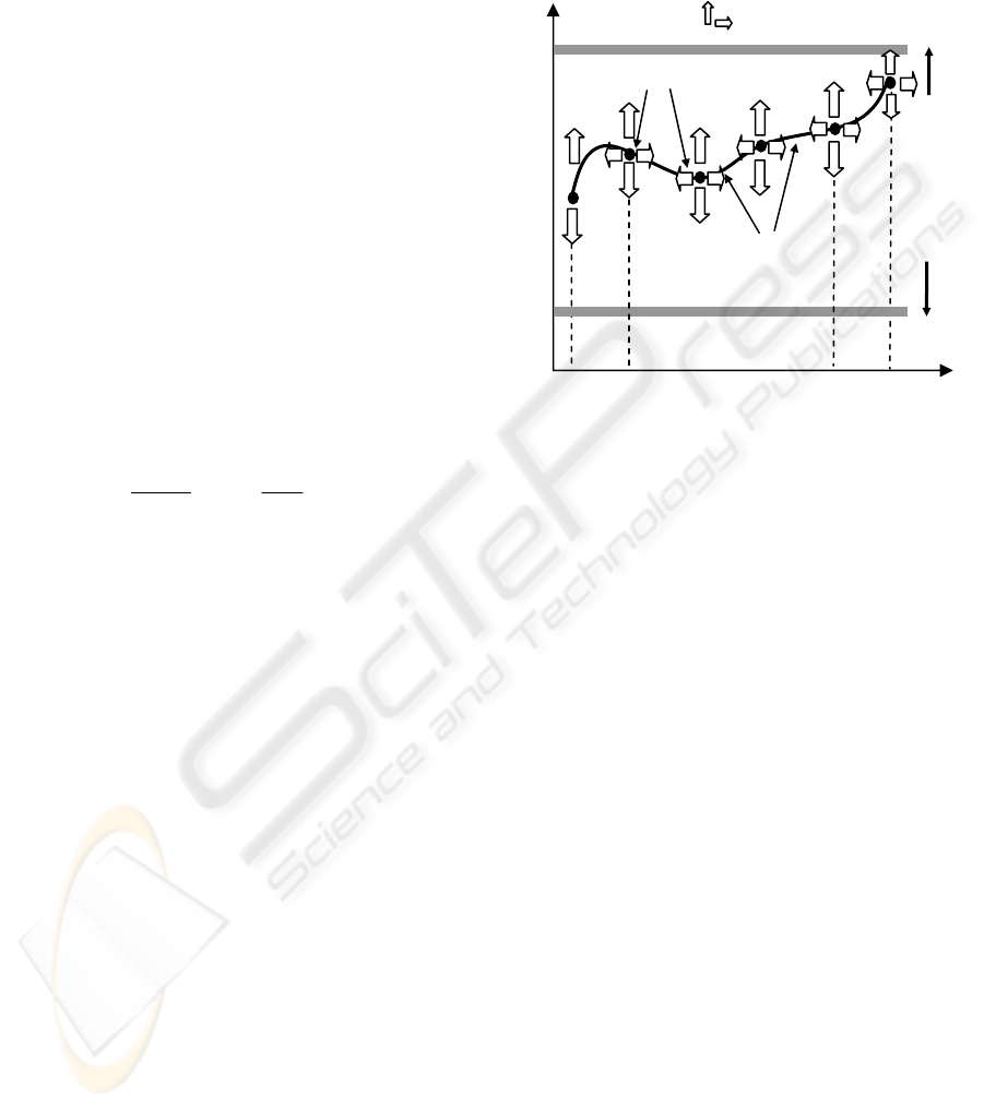
The conversion of the problem of trajectory
optimization into a POP starts with the definition of
N nodes (Knots), at fixed times,
Tttt
N
=<<<= ...0
21
, uniformly or not uniformly
distributed along the time scale. Then, the system’s
kinematic or dynamic continuous variables are
replaced by their values at the nodes (
kkk
qqq
,, or
k
τ
) and some form of interpolation (fig. 1). In
addition to final time parameter T, parameters of the
new parametric optimization problem can be chosen
in various ways as a combination of
kkk
qqq
,, or
k
τ
.
Along the optimization process, these parameters are
varied inside their admissible range until an
optimum minimizing the cost function and satisfying
all constraints has been reached. Examples of
methods for interpolating these knots (nodes) are
high-order polynomial and piecewise polynomials
(cubic- splines or B-splines).
Note that also the location of these nodes along the
time scale can be considered as additional unknowns
of our problem. The interest of this fact arises
particularly when we would like to capture critical
evolution areas like switching time for bang-bang
controls and, in consequence, to avoid excessive
refinement of the time grid.
If X denotes the set of chosen parameters, the
corresponding POP is to find the value of X that
minimizes the cost function (7) written here:
(
)
XFJ
X
=
min (10.a)
Subject to the equality constraints:
(
)
0
=
XC
eq
(10.b)
And the inequality constraints:
(
)
0
≤
XC
ineq
(10.c)
F, C
eq
and C
ineq
are just a transcription of relations
(4), (6) and (7) in terms of the new variable
X.
5.1 Conversion with independent
states and controls as unknowns
In this first mode of conversion, both the control
vector
τ
and state vector
() () ()
[]
t
tqtqtX
= are
discretized. This involves an implicit integration of
(4). This is performed by calculating the residuals on
each subinterval and driving them to zero as a part
of the optimization process. Hence we get additional
equality constraints. This discretization can be
f(t)
t
t
1
Nodes
Figure 1: Discretization of continuous system’s
variables.
Upper
bound
Admissible range
Lower
bound
An
interpolation
t
2
t
N-1
t
N
= T
Indicates possible
ii
ICINCO 2005 - ROBOTICS AND AUTOMATION
6

performed according different schemes: midpoint
rule, trapezoidal rule or in general using a Runge-
Kutta scheme (Hull,1997) (Betts,1999).
5.2 Conversion with Controls as
unknowns
In this conversion method, in addition to T, the
unknowns are the values of
τ
at the nodes. The
control history
τ
(t) is formed by interpolation. In this
case, the dynamic equation (1), written under the
state form (4), must be integrated on
[]
T,0 to get the
time evolution of the system state
()
(
)
(
)
[]
t
tqtqtX
=
(i.e. to compute the FDM). Such a method can be
seen as a shooting method because once a guess of
τ
(t) is made the sate equations are generally
integrated in one pass. So, the time history
τ
(t) is
varied until the final state (8
b) is matched while all
imposed constraints are respected and cost function
is optimized.
5.3 Conversion with independent
generalized coordinates as
unknowns
In this conversion method, T and the values of
independent generalized coordinates (defined from
q(t) at selected knots) are considered as the
unknowns of the problem. The time history of
q(t) is
then formed by interpolation. Time derivatives of
q(t), i.e. q
and q
, are systematically deduced. Then,
torques
τ
are computed using IDM (relation (1)). So,
all elements of the optimization problem, objective
function and constraints, can be easily evaluated and
then checked.
In this conversion, dynamic equations (1), exploited
through the IDM, are employed just to verify any
constraints imposed on torques
τ
. So, the motion
generator can be seen here as a conventional
kinematic planner.
6 SOLUTION TECHNIQUES
Once the original OCP has been transformed into a
POP using the above mentioned methods, the
problem can be treated by parametric optimization
techniques. These techniques can be regrouped into
two main families: deterministic and stochastic
techniques. Deterministic methods use first and
second order information (gradient and Hessian) to
build a descent direction and to define a good
progress step. In contrast, stochastic techniques need
neither gradient nor Hessian values to process the
optimization problem. They are based on
randomized process able to select good candidates.
We are not here going to establish a comparison
between these two families but, just we mention that
theses techniques can be used to solve the resulting
POP.
7 NUMERICAL EXAMPLES
7.1 A 2 d.o.f. robot
We are concerned here by the IBM 7535 B04 robot
modelled as a 2 d.o.f planar robot (Geering et al.,
1986). It was the bench mark for many simulation
works dealing with the minimum time trajectory
planning problem (Geering et al., 1986, Chen and
Desrochers, 1988, 1990, Chen et al, 1993,
Bessonnet, 1992, Lazrak, 1996). We try here to
solve this problem using parametric optimization
instead of Pontryagin Maximum Principle (PMP).
The three discretization schemes proposed in § 5 are
used to transform the original problem. Then, we
propose the SQP technique to solve the resulting NL
problem. In all cases, the task to be achieved is
characterized by null limit joint velocities while the
motion starts at (0, 0) and ends at (0, π/4). Only
constraints on torques are imposed
(
NmNm 9,25
21
≤≤
ττ
). Table 1 summarizes the
main simulation results we get using the three
conversion modes.
In the first conversion mode, the robot’s dynamic
model has been discretized using a mid-point rule
and using a uniform grid of 20 nodes. It has the
biggest number of variables and constraints.
However, the resolution of the corresponding NL
program does not involve the highest CPU time. In
fact, in the second mode of conversion, that involves
only 29 variables, we need more time (26 times vs
the first mode and 130 times vs the third mode) to
solve the NL program. This is basically due to the
fact that, at iteration of the optimization process, the
robot dynamic model (4) is integrated using standard
ODE solvers in order to get the corresponding
kinematics that is time consuming. In reality, in this
second mode, the optimization process behaves like
a shooting method. Once
τ
(t) is estimated inside the
admissible range, relation (1) is integrated from the
initial state to a final state that must meet the state
specified by the assigned task. This is traduced in
the program by four equality constraints. In contrast
to the two precedent modes, the last one seems to be
more efficient, we have less variables and a good
estimation of the optimal solution in a very short
PARAMETRIC OPTIMIZATION FOR OPTIMAL SYNTHESIS: of robotic systems’ motions
7
time (versus optimal solution for the same task
found using a PMP based method and given in
(Chen and Desrochers, 1990) that is 0.99s).
From this analysis, we think that the third mode is
much more efficient and robust to handle the
problem of trajectory optimization in more complex
situations. The two following examples attest and
confirm this point of view.
Table 1: Numerical results using direct and indirect
methods
Discretization
mode
Number of
parameters
Objective
function (s)
CPU
time (s)
1) τ, x
127 1.02 20
2) τ
29 1.14 525
3) q 5 1.05 4
PMP (Chen & Desrochers,1990) 0.99 -
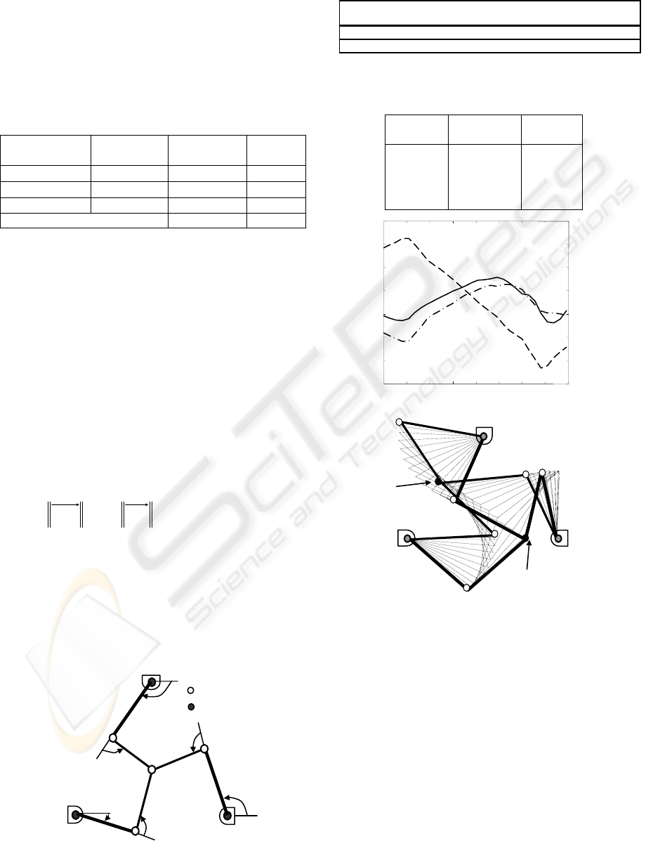
7.2 Optimal motion planning for a
closed chain robot
We consider here a 2-DOF planar parallel robot (fig.
2). It consists of three identical two-link legs
intersecting in a central point
C. The robot
configuration is defined by
[]
654321
,,,,, qqqqqq . Let
[]
321
,, qqqq
a
= corresponds to active joints and
[]
654
,, qqqq
p
=
to passive joints. The coordinates of
C are
()
[]
tytx ),( and can be expressed all the time
as a function of
q
a
and q
p
as follows:
() ( ) ( )
() ( ) ( )
3,...,1
sinsin
coscos
321
321
=
⎩
⎨
⎧
++=
++=
+
+
i
qqlqlty
qqlqltx
iii
iii
Where
1
lBA
ii
= ,
2
lCB
i
= .
So, the robot configuration can be parameterized
using only the two independents coordinates
x(t) and
y(t). Knowing
()
[]
tytx ),( and their time derivatives,
active joints’ torques can be computed using
adequate techniques proper to closed chain robots
(Cheng
et al., 2001). So, we decide to take
()
[]
tytx ),( as unknowns for the motion planning
problem.
Table 2: Characteristics of one leg of the redundant planar
parallel manipulator
Table 3: Numerical results for the Planar 2-DOF
redundant parallel robot.
µ
Cost
function(s)
Transfer
time(s)
0.25 0.52 1.58
0.50 0.80 1.21
0.75 0.96 1.07
1.00 1.04 1.04
The assigned task here consists to achieve a transfer
between an initial posture (
x=-0.3, y=0.2) and a final
one (
x=0.3, y=-0.3) while minimizing the objective
function (9) and respecting bounds (5
c) and (5g) on
the values of active joints’ positions and torques
(Table 2).
The time evolution of [
x(t), y(t)] is parameterized
using seven free nodes uniformly distributed along
the time scale. The simulation is done for various
j L
(m)
M
(kg)
d
(m)
Ι
(kg.m
2
)
τ
min
(N.m)
τ
max
(N.m)
q
min
(m)
q
max
(m)
1 0.6 10 0.3 0.1 -25 25
−0.5 0.5
2 0.6 10 0.3 0.1
− − −0.5
0.5
Figure 2: Planar 2-DOF redundant parallel mechanism
A
1
A
3
A
2
B
1
B
2
B
3
C
active joint
passive joint
q
2
q
1
q
3
q
4
q
5
q
6
0 0.2 0.4 0.6 0.8 1 1.2 1.4 1.6
-20
-15
-10
-5
0
5
10
15
Figure 3a
µ
=0.25
t(s)
τ
3
τ
1
τ
2
Figure 3: Simulation results for the Planar 2-DOF
redundant parallel robot: (a) active joint torques, (b)
optimised motion, for
µ
= 0,25
Figure 3b
Initial
configuration
final
configuration
ICINCO 2005 - ROBOTICS AND AUTOMATION
8
values of
µ
and corresponding results are reported in
Table 3 and depicted on figure 5.
We observe that the proposed method succeeds to
find a solution in both situations. Increasing the
coefficient
µ
means that we attempt to minimize
more
T, this is guaranteed by higher torques
amplitudes (increasing cost function). In fact, on fig.
5.a (
µ
=1), we note clearly the presence of several
saturation areas of active joints’ torques in order to
ensure high speed transfer (fig.5.
c). While, profiles
of fig.5.
b (
µ
=0.25) are quite smooth but the transfer
is executed slower (fig.5.
d).
Example 3: A mobile robot (Nonholonomic system)
This section gives numerical results concerning
minimum–time trajectories (
µ=1)
for a Wheeled
Mobile Robot
WMR constituted of a platform and
two independently driven wheels (Yamamoto
et al.,
1999). Constraints on driving torques are:
)(0.1,0.1
21
N.m ≤≤−
ττ
. The workspace consists
of a
mm 2424 × flat floor with three obstacles (Fig.
5
a). The WMR is required to move freely, without
following a specified path, from initial to final states
0
X
and
f
X
given by:
[][]
3 X 03
0000
===
T
yx
θ
,
[]
[]
6/2323
πθ
==
T
ffff
yxX
.
In addition to the vector
τ
a
(t) of actuator efforts and
the final time
T
, we must find the motion defined by
[]
T
ttytxt )()()()(
θ
=X
such as the initial and
final states are matched, constraints are respected
and the traveling time is minimized.
The robot independent position parameters are
x(t)
and y(t). The orientation
θ
(t) can be deduced from
the nonholonomic constraint:
() ()
0)()()()( =⋅+⋅− tCostytSintx
θ
θ
.
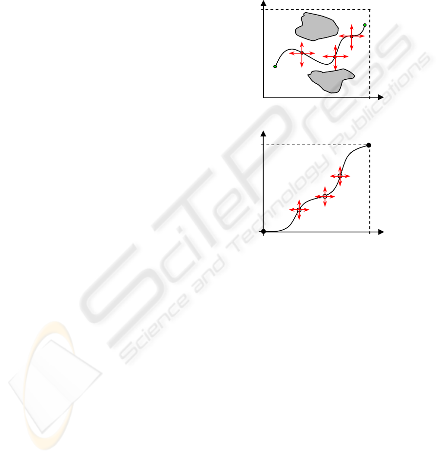
At each iteration of the optimization process the
WRM motion X(
t) is defined in two main steps.
Step
1 : specify the robot path X(λ).
Step
2 : specify the motion profile λ(ξ) on this path.
X(λ), λ ∈ [0, 1], describes the geometry of the robot
path in the (O, x, y)
plane while λ(ξ), ξ ∈ [0, 1],
determines the time evolution along this path (ξ
represents a normalized time scale: ξ =
t / T).
Hence, the problem is transformed to a parametric
optimization problem. One of the parameters is the
unknown traveling time
T. The other parameters are
two sets,
S
P
and S
C
, of free discretisation nodes. The
set
S
P
is composed of N
P
control points in the robot
workspace (Fig. 4
a) while S
C
consists of N
C
collocation points in the (ξ, λ) plane (Fig. 4
b). With
S
P
, we can define a path X(λ) using parametric
functions, such as B-spline, that takes into account
limit states. With
S
C
, we can define a motion profile
λ(ξ) using, for example, a clamped cubic spline
interpolation that takes into account the other
constraints (Chettibi et al 2004
b, Haddad et al,
2005).
The optimization method adopted here uses a
simulated annealing process that scans
simultaneously the available solution space of both
sets
S
P
and S
C
to propose candidate trajectory
profiles X(ξ) ≡ X(λ(ξ)) for a global minimization of
the traveling time.
For this problem we have adopted for X(λ) a fourth-
order B–spline model with
N
p
= 6 control points and
for λ(ξ) a clamped cubic spline model with
N
C
= 4
interpolation points. The required runtime was
about 4 minutes on a 2.4 GHz P4.
Simulation results are shown in Figure 5. These
results are quite similar to those given in
(Yamamoto
et al. 1999). The calculated traveling
times are of the same order (17.82 vs. 18.94
sec).
O
x
y
x
max
y
max
X
0
X
f
Obst.1
Obst.2
X(
λ
)
P
1
P
2
P
3
Figure 4a: A path X(
λ
) through N
P
free control points
(
ξ
1
,
λ
1
)
ξ
λ
1
0
1
(
ξ
2
, λ
2
)
(
ξ
3
, λ
3
)
Figure 4b: A motion profile λ(ξ) with N
C
free
collocation points
PARAMETRIC OPTIMIZATION FOR OPTIMAL SYNTHESIS: of robotic systems’ motions
9
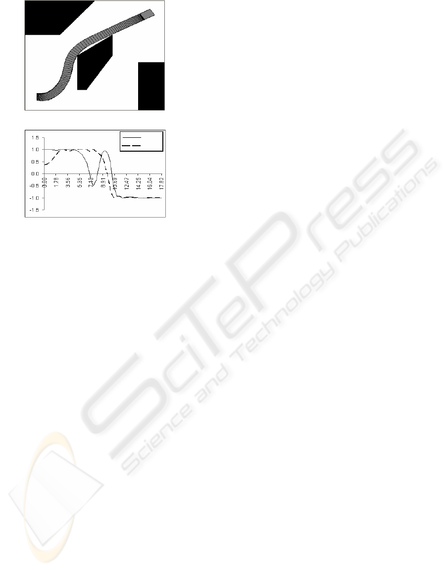
Figure 5b: Time evolution of joint torques
τ
[Nm]
τ
[1]
τ
[2]
Time
[
s
ec
]
Figure 5a: Simulation result
S
G
T
f
= 17.82
s
ec.
8 CONCLUSION
We have demonstrated that a trajectory optimization
problem, that is an optimal control problem, can be
converted into a parametric optimization problem
using three different conversion modes. We shown
that using independent position parameters as
principle variables of the optimization problem
offers many facilities and leads to comparable
results to those obtained heavy and classical indirect
methods.
Furthermore, the simplicity and the efficiency of this
conversion mode allow us to use it to solve the
problem of optimal trajectory planning in complex
situations, in particular for holonomic and non-
holonomic systems.
ACKNOWLEDGMENTS
Authors would like to thank Prof. H. E. Lehtihet for
his suggestions and helpful discussions.
REFERENCES
Angeles J., 1997, Fundamentals of robotic mechanical
systems. Theory, methods, and algorithms, Springer
Edition.
Ascher U. M. & Petzold L. R., 1998, Computer Methods
for ordinary differential equations and differential-
algebraic equations, SIAM edition.
Bessonnet, G. 1992. Optimisation dynamique des
mouvements point à point de robots manipulateurs.
Thèse d’état, Université de Poitiers, France.
Betts, J. T. 1998. Survey of numerical methods for
trajectory optimization. Jour. Of Guidance, Cont. and
Dyn., 21(2), 193-207.
Bryson A. E., 1999, Dynamic Optimization, Addison
Wesley Longman, Inc.
Bicchi A., Pallottino L., Bray M., Perdomi P. , 2001,
Randomized parallel Simulation of constrained
multibody systems for VR/Haptic applications, Proc.
IEEE int. conf. on rob. & Aut., Korea.
Bobrow, J. E., Martin, B. J., Sohl, G., Wang, E. C., Park,
F. C., and Kim, J. 2001. Optimal robot motions for
physical criteria. Jour. Of Rob. Syst. 18 (12), 785-795.
Chen, Y., and Desrochers, A. 1990. A proof of the
structure of the minimum time control of robotic
manipulators using Hamiltonian formulation. IEEE
Trans. On Rob. and Aut. 6(3), pp388-393.
Chettibi T., H. E. Lehtihet, M. Haddad, S. Hanchi, 2004a,
Minimum cost trajectory planning for industrial
robots, European Journal of Mechanics/A, pp703-715.
Chettibi T., Haddad M., Rebai S., Hentout A., 2004b, A
Stochastic off line planner of optimal dynamic
motions for robotic manipulators, 1
st
Inter. Conf. on
Informatics, in Control, Automation and Robotics,
Portugal.
Dombre E. & Khalil W., 1999, Modélisation,
identification et commande des robots, second edition,
Hermes.
Geering, H. P., Guzzella, L., Hepner, S. A. R., and Onder,
C. H. 1986. Time-optimal motions of robots in
Assembly tasks. IEEE Trans. On Automatic control ,
Vol. AC-31, N°6.
Haddad M., Chettibi T., Lehtihet H. E. and Hanchi S.
2005. “A new approach for minimum time motion
planning problem of wheeled mobile robots”, accepted
at the 2005IFAC congress, Prague.
Hull, D. G. 1997. Conversion of optimal control problems
into parameter optimization problems, Jour. Of
Guidance, Cont. and Dyn., 20(1), 57-62.
Lazrak, M. 1996. Nouvelle approche de commande
optimale en temps final libre et construction
d’algorithmes de commande de systèmes articulés.
Thèse d’état, Université de Poitiers.
Steinbach M.C., 1995, Fast recursive SQP methods for
large scale optimal control problem. PhD thesis,
Universität Heidelberg.
Stryk, O. V. and Bulirsch R. 1993. Direct and indirect
methods for trajectory optimization. Annals of
Operations research, Vol 37, pp. 357-373.
Stryk, O. V. 1993, Numerical solution of optimal control
problems by direct collocation. Optimal control theory
and numerical methods, Int. series of Numerical
Mathematics, Vol 111, pp 129-143.
Yamamoto, M., Iwamura M. and Mohri A. (1999). Quasi-
time-Optimal Motion Planning of Mobile Platforms in
the presence of obstacles, Proc. Of 1999 IEEE ICRA,
2958-2962.
ICINCO 2005 - ROBOTICS AND AUTOMATION
10
