
DISCRETE–TIME FREE AND FIXED END-POINT OPTIMAL
CONTROL PROBLEM
Corneliu Botan, Florin Ostafi
Department of Automatic Control and Industrial Informatics, Technical University of Iasi, Blvd D. Mangeron 53A, Iasi,
Romania
Keywords: Optimal control, Linear quadratic, Discrete, Fixed, Free end-point.
Abstract: A comparison between the fixed and free end-point discrete time linear quadratic optimal problem is
performed. Symmetrical algorithms for both problems are proposed. These algorithms can be easier
implemented by comparison with classical procedures. Simulation results are presented.
1 INTRODUCTION
The paper considers the discrete time optimal
problems with finite final time, which refer to a
quadratic criterion and to a discrete completely
controllable linear time invariant system
x(k 1) Ax(k) Bu(k)+= + (1)
where
n
x(k)∈ \ is the state vector,
m
u(k)∈ \ is the
control vector,
k ∈ ] , A and B are matrices of
appropriate dimensions.
Depending on the final state x(k
f
), one can formulate
the following problems:
P1 (with fixed end-point): Find the feedback control
u(x(k)) which transfers the system (1) from the
initial state x(k
0
) in the imposed final state x(k
f
)=0
and minimizes the criterion
f
0
k
TT
111
kk
1
J x (k)Q x(k) u (k)Pu(k)
2
=
=+
∑
(2)
(T denotes the transposition).
P2 (with free end–point): Find the optimal feedback
control u(x(k)) which transfers the system (1) from
the initial state x(k
0
) in the free final state x(k
f
) and
minimizes the criterion
f
0
k
TTT
2ff 1 1
kk
11
J x (k )Sx(k ) x (k)Q x(k) u (k)Pu(k)
22
=
=+ +
∑
(3)
We also mention in addition the problem P3 with
infinite final time, which refers to the criterion
TT
333
k0
1
J x (k)Q x(k) u (k)P u(k)
2
∞
=
=+
∑
(4)
For a more relevant comparison we shall consider
123
QQQQ
=
==,
123
PPPP
=
== (5)
The matrices of the above criteria are
symmetrical and
S0,Q0,P0≥≥> (6)
The solution for the above formulated problems
are well known (Anderson, Moore, 1990), (Kuo,
1992), but there are some difficulties in
implementation of the algorithms. The solution to
the P1 problem is usually presented as an open loop
control u(k) because the feedback control u(x(k)) has
a complicated form. The P2 problem is the most
frequently meet linear quadratic problem with finite
final time. The matrix of the feedback controller is
time variant and is designed based on a solution to
the Riccati difference matriceal equation. This
solution has to be computed in real time and this fact
can generate some difficulties in implementation,
augmented by the fact that the equation must be
solved in inverse time, starting from a final
condition.
170
Botan C. and Ostafi F. (2005).
DISCRETE–TIME FREE AND FIXED END-POINT OPTIMAL CONTROL PROBLEM.
In Proceedings of the Second International Conference on Informatics in Control, Automation and Robotics, pages 170-175
DOI: 10.5220/0001158301700175
Copyright
c
SciTePress

The paper uses some previous results of the
authors (Botan, Onea, 1999), (Botan, Ostafi, Onea,
2003), and presents a simpler for implementation
solution for the formulated problems. Moreover, a
symmetrical approach for both problems is
established.
2 USUAL APPROACHES
From the Hamilton necessary conditions, the optimal
control is obtained as
1T
u(k) P B (k 1)
−
=− λ +
(7)
and
T
Qx(k) A (k 1) (k)+λ+=λ, (8)
where
n
(k)λ∈\
is the co-state vector.
Substituting
(k 1)λ+ from (8) in (7) and then in
(1), the equations (1) and (8) can be expressed as
(k 1) G (k)γ+=γ ,
2n
x(k)
(k)
(k)
⎡⎤
γ= ∈
⎢⎥
λ
⎣⎦
\
, (9)
where
TT
TT
ANAQ NA
G
AQ A
−−
−−
⎡⎤
+−
=
⎢⎥
−−
⎣⎦
(10)
with
1T
NBPB
−
= and
TT1
A(A)
−−
= .
The solution to the system (9) is
00
11 0 12 0 0
21 0 22 0 0
x(k)
(k) (k,k ) (k )
(k)
(k,k) (k,k) x(k)
(k, k ) (k, k ) (k )
⎡⎤
γ= =Γ γ
⎢⎥
λ
⎣⎦
ΓΓ
⎡⎤⎡⎤
=
⎢⎥⎢⎥
ΓΓλ
⎣⎦⎣⎦
(11)
where
(.)Γ is the transition matrix for G.
The next steps are different for the
P1 and P2
problems, depending on terminal conditions:
- in the
P1 problem x(k
0
) and
f
x(k ) 0= (12)
are imposed (
λ(k
0
) and λ(k
f
) are free);
- in the
P2 problem x(k
0
) and
ff
(k ) Sx(k )
λ
= (13)
(from the transversallity condition) are imposed
(x(k
f
) and λ(k
0
) are free).
Thus, for the
P1 problem, from (11) and (12), it
results
00
(k ) Lx(k )
λ
= ,
1
12f011f0
L(k,k)(k,k)
−
=Γ Γ (14)
It was proved (Botan, Ostafi, Onea, 2003) that
1
12 f 0
(k ,k )
−
Γ is a non-singular matrix if the system (1)
is completely controllable. Note also that all inverse
matrices which appear in the following equations are
non singular.
Therefore,
0
(k )
γ
is known and the solution (11)
can be obtained. Then it is possible to express u(k)
in terms of
0
x(k ) , starting from (7). This expression
offers the open loop control u(k) and it is the usual
solution presented in the literature. It is possible to
obtain the feedback control u(x(k)) if x(k
0
) is
expressed in terms of x(k). The formula is
complicated and contains the inverse of a time
variant matrix and this fact introduces great
difficulties in the real time implementation.
A similar procedure can be used for the
P2
problem, but in this case it is preferred another way,
namely imposing
(k) R(k)x(k)λ=
, where R(k)
is
obtained as a solution to a Riccati difference
matriceal equation. The difficulties which arise in
this case were mentioned above.
3 MAIN RESULTS
A significant simplification is obtained if we
perform a change of variables:
(k) U (k)
γ
=ρ (15)
with
I0
U
RI
⎡
⎤
=
⎢
⎥
⎣
⎦
,
1
I0
U
RI
−
⎡⎤
=
⎢⎥
−
⎣⎦
(16)
where I is the nxn identity matrix and R is a
symmetrical nxn matrix. According to (15) and (16),
the new system is
(k 1) H (k)
ρ
+=ρ , (17)
where
DISCRETE–TIME FREE AND FIXED END-POINT OPTIMAL CONTROL PROBLEM
171

11 12
1
21 22
HH
HUGU
HH
−
⎡⎤
==
⎢⎥
⎣⎦
(18)
and
x(k)
(k)
v(k)
⎡⎤
ρ=
⎢⎥
⎣⎦
,
v(k) (k) Rx(k)=λ − (19)
Using (10), (16) and (18), it is obtained by
straightforward computing
21 11 12 21 22
TT1
HRGRGRGGR
(I RN)A [R Q A (I RN) RA]
−−
=− − + +
=+ −− +
(20)
If we impose the condition
T1
RQA(IRN)RA
−
=+ +
, (21)
then
21
H0= (22)
(Note that (21) is the Riccati matriceal equation for
the
P3 problem). The others matriceal blocks of H
can be similarly computed. Using in addition (21),
yields
1
11 11 12
HGGR[IN(INR)R]A
−
=+ =−+
,
or
1
11
H(INR)A
−
=+ ,
T
12 12
HG NA
−
==−
TT
22 12 22 11
H RG G (I RN)A H
−−
=− + = + = (23)
The solution to the equation (17) is
00
x(k)
(k) (k,k ) (k )
v(k)
⎡⎤
ρ= =Ω ρ
⎢⎥
⎣⎦
, (24)
where (for k
0
=0)
11 0 12 0
k
0
22 0
(k,k ) (k,k )
(k,k ) H
0(k,k)
ΩΩ
⎡⎤
Ω==
⎢⎥
Ω
⎣⎦
(25)
is the transition matrix for H.
Using (16) and (18), yields
kk
11 11 22 22
k1
iki1
12 12k 11 12 22
i0
(k) H , (k) H
(k) H H H H
−
−−
=
Ω=Ω=
Ω==
∑
(26)
From (17), (22), (24) and (26) it results (for k
0
=0)
22
22 0 22 0
k
v(k 1) H v(k) and
v(k) (k)v(k ) H v(k )
+=
=Ω =
(27)
The optimal control results from (7) and (19)
1T
u(k) P B [Rx(k 1) v(k 1)]
−
=
−+++
Using (17) and (27), we can write
f
s
u(k) u (k) u (k)
=
+ , (28)
where u
f
(k) is a feedback component
1T
f11
u (k) P B RH x(k)
−
=−
(29)
and u
s
(k) is a supplementary component, given by
1T
12 22
s
u (k) P B (RH H )v(k)
−
=− + , (30)
with v(k) given by (27).
Remark 1: For the problem with infinite final time,
the vector u(k) contains only the feedback
component u
f
(k) given by (29).
In order to establish the supplementary
component with (30), we have to express v(k
0
) in
terms of x(k
0
), which is the unique known terminal
condition.
These operations are different for the two problems.
For
P1 problem:
From (15) and (20) one obtain
00
v(k ) (L R)x(k )
=
− . (31)
Using
1
UU
−
Γ= Ω , we obtain
11 0 11 0 12 0
(k,k ) (k,k ) (k, k )R
Γ
=Ω −Ω ,
12 0 12 0
(k,k ) (k,k )
Γ
=Ω
and then, it results from (14)
ICINCO 2005 - INTELLIGENT CONTROL SYSTEMS AND OPTIMIZATION
172

1
12 f 0 11 f 0
L(k,k)(k,k)R
−
=Ω Ω + (32)
and one obtain from (31)
f
f
1
012f011f00
k
1
11k 11 0
v(k) (k,k) (k,k)x(k)
HHx(k)
−
−
=−Ω Ω
=
(33)
For
P2 problem:
Using (13) and (19), yields
ff
v(k) (S R)x(k)=− . (34)
From (24) and (25)
f22f00
v(k ) (k , k )v(k )=Ω
,
so that
1
022f0 f
v(k ) (k ,k )(S R)x(k )
−
=Ω − . (35)
We can write from (24)
f11f0012f00
x(k ) (k ,k )x(k ) (k ,k )v(k )=Ω +Ω
and using (35), we obtain
f0
x(k ) Mx(k )= , (36)
where M is a constant nxn matrix
11
12 f 0 22 f 0 11 f 0
M [I (k ,k ) (k ,k )] (k ,k )
−−
=−Ω Ω Ω
(37)
Finally, from (35) we can write
1
022f0 0
v(k ) (k ,k )(S R)Mx(k )
−
=Ω − (38)
Remark 2: Unlike the usual methods which solve the
P1 and P2 problem by different ways, a symmetrical
approach was proposed for the two problems. A
similar equation (28) for the optimal control u(k)
was obtained for the problems
P1 and P2. In both
cases, u(k) contains a feedback component u
f
(k) (29)
and a supplementary one u
s
(k) (30). Note that the
feedback component is the same in
P1, P2 and P3
problems. The component u
s
(k) depends on the
vector v(k) given by (27). The difference between
the two problems consists in the expression of the
initial value v(k
0
): (33) for the P1 problem and (38)
for the
P2 problem.
Remark 3: Some of the above established equations
are rather complicated, but the most part of the
computation is performed off-line, in the stage of
controller design. It is important that the real time
computing implies only to establish the components
u
f
(k) and u
s
(k) given by (29) and (30), respectively.
Therefore, the real time computing volume does not
exceed very much the usual state feedback control.
Moreover, the supplementary component can be
recurrently computed. Indeed, the vector v(k) which
appears in (30) can be recurrently computed, as it is
indicated in (27), with the initialisation v(k
0
) given
by (33) or (38) for the
P1 and P2 problems,
respectively.
4 SIMULATION RESULTS
Some simulation tests were performed for both P1
and P2 problems. The following discrete completely
controllable linear time invariant system was
considered (the example is applicable to a servo
drive system):
1 0.0002 0 0
x(k 1) 0 1 0.04 x(k) 0.0002 u(k)
0 -0.007 0.962 0.0123
⎡⎤⎡⎤
⎢⎥⎢⎥
+= +
⎢⎥⎢⎥
⎢⎥⎢⎥
⎣⎦⎣⎦
The matrices in the criteria (2) and (3) are:
10 0
Q00.50
003.1
⎡
⎤
⎢
⎥
=
⎢
⎥
⎢
⎥
⎣
⎦
,
1000 0 0
S010
000
⎡⎤
⎢⎥
=
⎢⎥
⎢⎥
⎣⎦
, P=p=1
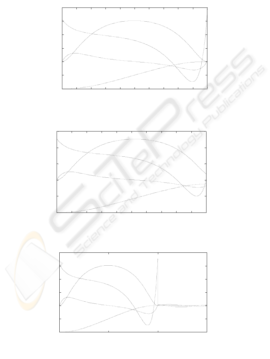
The Figure 1 and Figure 2 show the behaviour of the
optimal system in the case of the LQ problem with
fixed end-point and with free end-point,
respectively. In the both simulations t
0
= 0 s (k
0
=0),
t
f
= 1s (k
f
=500), the sampling period τ=0.002 s,
x
0
=[-2 0 0]
T
.
Generally, the optimal control refers to a specified
time interval. If we are interested to maintain the
desired state after the final time t
f
= k
f
τ, the control
law u(k) must be changed for k>k
f
. For the
mentioned example, the control law was changed as
12 f
u(k) x (k) x (k), k k
=
−α −β > , α>0, β>0
where x
1
(k) and x
2
(k) are the two first state variables
(corresponding to the position and to the speed, if
we refer to a servo system) If it is necessary, a
DISCRETE–TIME FREE AND FIXED END-POINT OPTIMAL CONTROL PROBLEM
173
discrete low pass filter can be introduced in order to
avoid an abrupt change of u(k) at the moment k
f
.
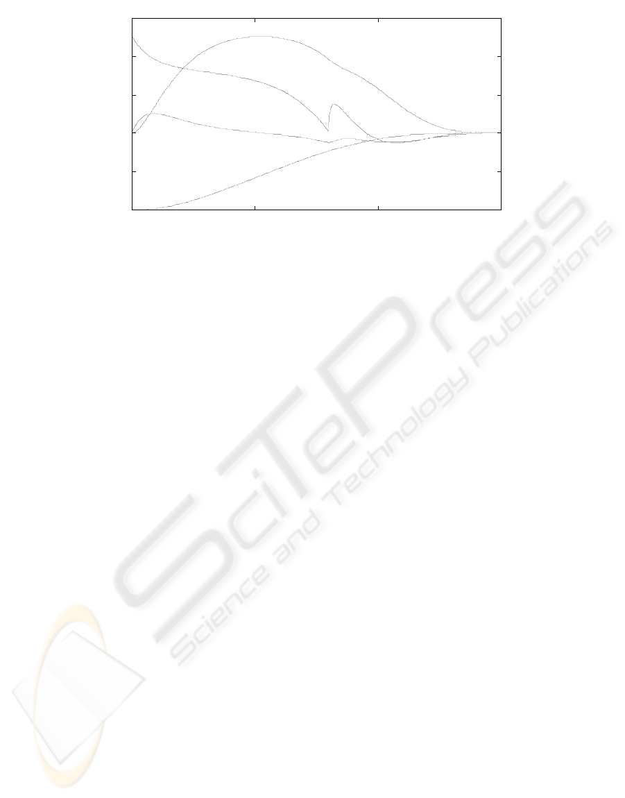
The behaviours in the case of the change of the
optimal control law at the moment t
f
are presented in
the figures 3 and 4, for
P1 and P2 problems,
respectively (the change of the control law for the
P2 problem was performed for k>0.8k
f
).
Fi
g
ure 2: The behaviour of the o
p
timal s
y
stem in the case of the L
Q
p
roblem with free en
d
-
p
oint
0 0.1 0.2 0.3 0.4 0.5 0.6 0.7 0.8 0.9 1
-20
-10
0
10
20
30
time
[
s
]
x
2
u
x
3
10*x
1
0 0.1 0.2 0.3 0.4 0.5 0.6 0.7 0.8 0.9 1
-20
-10
0
10
20
30
40
time
[
s
]
x
2
u
x
3
10*x
1
Fi
g
ure 1: The behaviour of the o
p
timal s
y
stem in the case of the L
Q
p
roblem with fixed en
d
-
p
oint
0 0.5 1 1.5
-20
-10
0
10
20
30
40
time
[
s
]
x
2
u
x
3
10*x
1
Figure 3: The behaviour of the optimal system for t<t
f
and for t>t
f
(t
f
=1s) in the case of P1 problem
ICINCO 2005 - INTELLIGENT CONTROL SYSTEMS AND OPTIMIZATION
174
In both simulated cases (for k<k
f
and k>k
f
), it was
calculated
2
u(k)
∑
and one can remark that this
value is bigger in the case of the
P1 problem (with
35%, approximately). This result is expected
because in this case the system is forced to reach the
imposed final state x(k
f
)=0.
As it was mentioned, the proposed algorithms can be
easier implemented as the classical procedure. Using
the MATLAB functions TIC and TOC, the
computing time was established. In the case of
mentioned example, for all operations performed in
a sampling period, it was obtained about 0.06 ms for
both
P1 and P2 problems in the case of the proposed
algorithm. In the same conditions, the computing
time was 2.6 and 4.6 times grater for the
P1 and P2
problem, respectively, if a classical approach was
used.
5 CONCLUSIONS
A comparison between LQ optimal problems with
fixed end-point and free end-point is performed.
By comparison with classical procedures,
thealgorithms proposed in the paper for the both
problems have advantages and lead to a significant
decrease of the computing time.
For the both problems, the proposed approach
leads to a similar solution: the optimal control
contains similar feedback and supplementary
components; the difference is between the last
components, which involve different initialisation
for a vector.
REFERENCES
Anderson, B.D.O., J.B. Moore, 1990. Optimal Control,
Prentice-Hall, Englewood Cliffs, New Jersey.
Kuo, B.C., 1992 Digital Control System, Saunders College
Publishing, Philadelphia.
Boţan C., Onea A., 1999. A Fixed End-Point Problem for
an Electrical Drive System. Proceedings of the IEEE
International Symposium on Industrial Electronics,
ISIE’99, Bled, Slovenia, , Vol. 3, pp. 1345-1349.
Boţan C., Ostafi F., Onea A., 2003. A Solution to the
Fixed End-Point Problem. Advances in Automatic
Control, Ed.: M. Voicu, Kluver Academic Publishers,
Boston/Dordrecht/London, pp. 9-20, ISBN: 1-4020-
7607-X.
Figure 4: The behaviour of the optimal system for t<t
f
and for t>t
f
(t
f
=1s) in the case of P2 problem
0 0.5 1 1.5
-20
-10
0
10
20
30
time
[
s
]
x
2
u
x
3
10*x
1
DISCRETE–TIME FREE AND FIXED END-POINT OPTIMAL CONTROL PROBLEM
175
