
PERFORMANCE ANALYSIS OF TIMED EVENT GRAPHS WITH
MULTIPLIERS USING (Min, +) ALGEBRA
Samir Hamaci
Jean-Louis Boimond
S
´
ebastien Lahaye
LISA
62 avenue Notre Dame du Lac - Angers, France
Keywords:
Timed event graphs with multipliers, (min,+) algebra, linearization, cycle time.
Abstract:
We are interested in the performance evaluation of timed event graphs with multipliers. The dynamical equa-
tion modelling such graphs are nonlinear in (min,+) algebra. This nonlinearity is due to multipliers and pre-
vents from applying usual performance analysis results. As an alternative, we propose a linearization method
in (min,+) algebra of timed event graphs with multipliers. From the obtained linear model, we deduce the
cycle time of these graphs. Lower and upper linear approximated models are proposed when linearization
condition is not satisfied.
1 INTRODUCTION
Timed event graphs (TEG’s) are well adapted to
model synchronization phenomena occuring in dis-
crete event systems (Murata, 1989). Their behav-
ior can be modelled by recurrent linear equations in
(min, +) algebra (Baccelli et al., 1992). When the size
of the model becomes very significant, techniques of
analysis developed for these graphs reach their limits.
A possible alternative consists in using timed event
graphs with multipliers, denoted TEGM’s. Indeed,
the use of multipliers associated with arcs is natural
to model a large number of systems, for example,
when the achievement of a specific task requires sev-
eral units of a same resource, or when an assembly
operation requires several units of a same part.
To our knowledge, few works deal with the per-
formance analysis of TEGM’s. In fact, in the most
of works the proposed solution is to transform the
TEGM into an ordinary TEG, which allows the use
of well-known methods of performances analysis.
In (Munier, 1993) the initial TEGM is the object
of an operation of expansion. Unfortunately, this
expansion can lead to a model of significant size,
which does not depend only on the initial structure
of the TEGM, but also on initial marking. With this
method, the system transformation proposed under
single server semantics hypothesis, or in (Nakamura
and Silva, 1999) under infinite server semantics hy-
pothesis, leads to a TEG with |θ| transitions (|θ| is
the 1-norm of the elementary T-semiflow of the cor-
responding TEGM).
Another linearization method was proposed in
(Trouillet et al., 2002) when each elementary circuit
of graph contains at least one normalized transition
(i.e., a transition for which its corresponding elemen-
tary T-semiflow component is equal to one). This
method increases the number of transitions. Inspired
by this work, a linearization method without increas-
ing the number of transition was proposed in (Hamaci
et al., 2004).
A calculation method of cycle time of a TEGM is
proposed in (Chao et al., 1993) but under restrictive
conditions on initial marking.
The weights on the arcs of a TEGM are nonlinearly
modelled in (min, +) algebra. Based on works given in
(Cohen et al., 1998), we propose a new method of lin-
earization without increasing the number of transition
from the graph. The obtained (min, +) linear model
allows to evaluate the performance of these graphs.
According to initial marking, these performances are
evaluated in an exact or approached way.
This article is organized as follows. Some concepts
on TEGM’s and their functioning are recalled in Sec-
tion 2. The method of linearization is presented in
Section 3. From the equivalent, or approached, TEG
of a TEGM, we deduce the cycle time in the Section
4.
16
Hamaci S., Boimond J. and Lahaye S. (2005).
PERFORMANCE ANALYSIS OF TIMED EVENT GRAPHS WITH MULTIPLIERS USING (Min, +) ALGEBRA.
In Proceedings of the Second International Conference on Informatics in Control, Automation and Robotics - Signal Processing, Systems Modeling and
Control, pages 16-21
DOI: 10.5220/0001157700160021
Copyright
c
SciTePress
2 RECURRENT EQUATIONS OF
TEGM’s
We assume that the reader is familiar with the
structure, firing rules, and basic properties of Petri
nets, see (Murata, 1989) for more details.
Consider a Petri net defined as a valued bipartite
graph given by a five-tuple (P, T, M, m, τ ) in which:
• P and T represent the finite set of places, and
transitions respectively;
• A multiplier M is associated with each arc. Given
q ∈ T and p ∈ P, the multiplier M
pq
(respectively,
M
q p
) specifies the weight (in N) of the arc from
transition q to place p (respectively, from place p to
transition q). A zero value for M codes an absence
of arc;
• With each place are associated an initial marking
(m
p
assigns an initial number of tokens (in N) in
place P) and a holding time (τ
p
gives the minimal
time (in N) a token must spend in place p before
it can contribute to the enabling of its downstream
transitions).
We denote by
•
q (resp., q
•
) the set of places
upstream (resp., downstream) transition q. Similarly,
•
p (resp., p
•
) denotes the set of transitions upstream
(resp., downstream) place p.
An event graph is a Petri net whose each place has
exactly one upstream and one downstream transition.
We denote W the incidence matrix of a Petri net.
A vector θ ∈ N
T
such that θ 6= 0 and W θ = 0 is a
T-semiflow. A T-semiflow θ has a minimal support
iff there exists no other T-semiflow, θ
′
, such that
{q ∈ T | θ
′
(q) > 0} ⊂ {q ∈ T | θ(q) > 0}.
A vector Y ∈ N
P
such that Y 6= 0 et Y
t
W = 0 is
a P-semiflow.
In the rest of the paper we assume that TEGM’s are
consistent (i.e., there exists a T-semiflow θ covering
all transitions : kθk = T) and are conservative (i.e.,
there exists a P-semiflow Y covering all places:
kY k = P ).
Remark 1 We disregard without loss of generality
firing times associated with transitions of a TEG be-
cause they can always be transformed into holding
times on places (Baccelli et al., 1992, §2.5).
With each transition q is associated a counter
variable, denoted n
q
: n
q
is an increasing map from
R to Z ∪ {+∞}, t 7→ n
q
(t) which denotes the
cumulated number of firings of transition q up to time
t.
In the following, we assume that counter variables
satisfy the earliest firing rule, i.e., a transition q fires
as soon as all its upstream places {p ∈
•
q} contain
enough tokens (M
q p
) having spent at least τ
p
units of
time in place p. When the transition q fires, it con-
sumes M
q p
tokens in each upstream place p and pro-
duces M
p
′
q
tokens in each downstream place p
′
∈ q
•
.
Assertion 1 The counter variable n
q
of a TEGM (un-
der the earliest firing rule) satisfies the following tran-
sition to transition equation:
n
q
(t) = min
p∈
•
q , q
′
∈
•
p
⌊M
−1
q p
(m
p
+ M
pq
′
n
q
′
(t − τ
p
))⌋.
(1)
Let us note the presence of inferior integer part to
preserve integrity of Eq. (1). In general, a transition
q may have several upstream transitions ({q
′
∈
••
q})
which implies that its associated counter variable is
given by the min of transition to transition equations
obtained for each upstream transition.
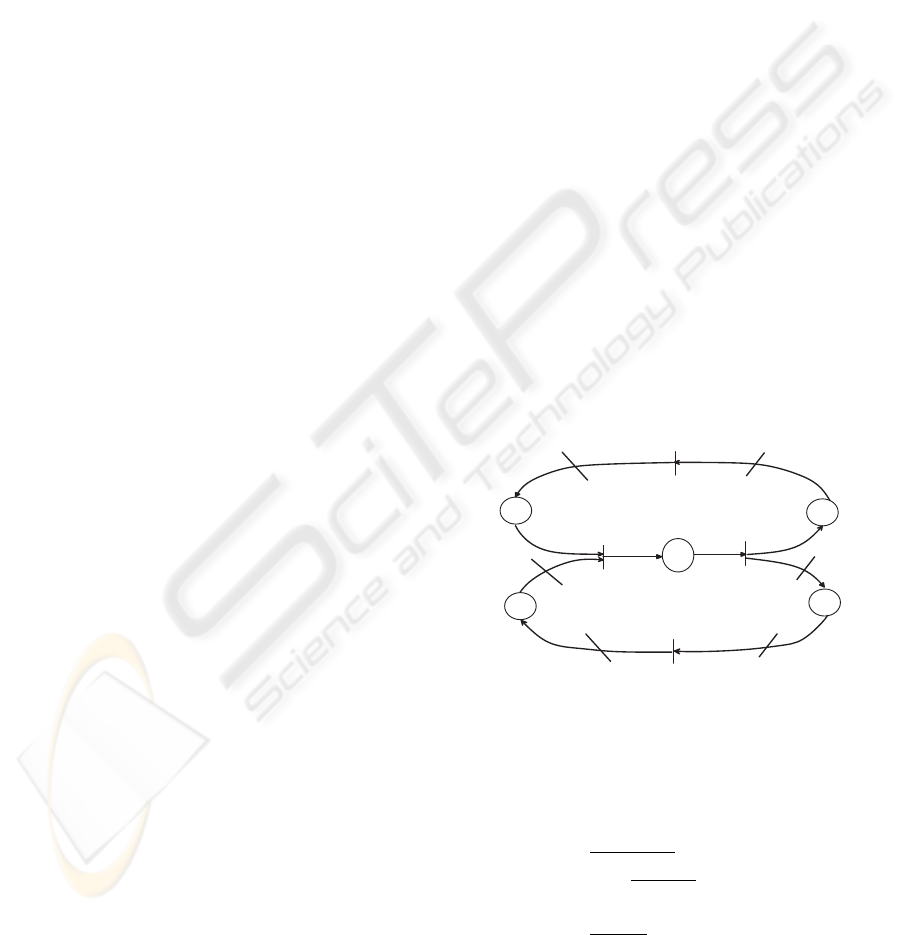
Example 1
n 3
n 4
n 2
n 1
6
3
1
2
3
1
P 1
P 3
P 2
P 4
P 5
1
3
3
3
3
2
2
Figure 1: A TEGM.
The counter variables associated with transitions of
TEGM depicted in the figure 1 satisfy the next system
equations:
n
1
(t) = ⌊
6+2n
3
(t−1)
3
⌋,
n
2
(t) = min(⌊
3n
1
(t−2)
2
⌋, 3 + 3n
4
(t − 3)),
n
3
(t) = n
2
(t − 1),
n
4
(t) = ⌊
n
3
(t−1)
3
⌋.
In the case of ordinary TEG’s, the transition to
transition equation given in Eq. (1) becomes:
PERFORMANCE ANALYSIS OF TIMED EVENT GRAPHS WITH MULTIPLIERS USING (Min, +) ALGEBRA
17

x
q
(t) = min
p∈
•
q , q
′
∈
•
p
(m
p
+ x
q
′
(t − τ
p
)). (2)
This equation is linear in the algebraic structure
called (min, +) algebra. This structure, denoted Z
min
,
is defined as the set Z ∪ {+∞}, equipped with the
min as additive law (denoted ⊕) and with the usual
addition as multiplicative law (denoted ⊗). The
neutral element of the law ⊕ (resp., ⊗) is denoted
ε = +∞ (resp., e = 0). More generally, the (min, +)
algebra is a dioid (Baccelli et al., 1992).
A dioid (D, ⊕, ⊗) is a semiring in which ⊕ is
idempotent (∀a, a ⊕ a = a). Neutral elements of ⊕
and ⊗ are denoted ε and e respectively.
From the Eq.(2) obtained for each transition, one
can express a TEG as the following recursive matrix
equation:
x(t) = A ⊗ x(t − 1), (3)
where A is a square matrix with coefficient in Z
min
,
and x(t) is the vector of the counter variables associ-
ated with transitions of the graph. See (Baccelli et al.,
1992) for more details on the representation of TEG’s
in the dioid Z
min
.
3 LINEARIZATION OF TEGM’S
A TEGM is linearizable if there exists a change of
variable n
q
(t) = θ
q
x
q
(t) such that x
q
(t) satisfies a
(min,+) linear recurrent equation knowing that:
• n
q
(t) is the counter associated with transition q of
TEGM,
• θ
q
is the component of T-semiflow associated with
transition q (θ
q
∈ N
∗
).
Proposition 1 A TEGM is linearizable if
∀q ∈ T, ∀p ∈
•
q, ⌊
m
p
M
q p
⌋ ∈ θ
q
N. (4)
Proof: According to assertion (1), we have for
each transition q of a TEGM:
n
q
(t) = min
p∈
•
q , q
′
∈
•
p
⌊M
−1
q p
(m
p
+ M
pq
′
n
q
′
(t − τ
p
))⌋.
Using the change of variable n
q
(t) = θ
q
x
q
(t), and
by distributivity of the multiplication with respect to
the min operator, we have:
x
q
(t) = min
p∈
•
q , q
′
∈
•
p
1
θ
q
⌊(
m
p
M
qp
+
M
pq
′
M
qp
n
q
′
(t − τ
p
))⌋.
From relation
θ
q
M
pq
′
=
θ
q
′
M
qp
, obtained for consistent and conserv-
ative TEGM (see (Munier, 1993)), we have
x
q
(t) = min
p∈
•
q , q
′
∈
•
p
1
θ
q
⌊(
m
p
M
qp
+
θ
q
θ
q
′
n
q
′
(t − τ
p
))⌋,
i.e.,
x
q
(t) = min
p∈
•
q , q
′
∈
•
p
1
θ
q
⌊(
m
p
M
qp
+ θ
q
x
q
′
(t − τ
p
))⌋.
Because θ
q
x
q
′
(t − τ
p
) ∈ N, we finally obtain
x
q
(t) = min
p∈
•
q , q
′
∈
•
p
(
1
θ
q
⌊
m
p
M
q p
⌋ + x
q
′
(t − τ
p
)), (5)
which corresponds to a (min,+) linear recurrent
equation.
More generally, if the condition (4) is satisfied for
each transition, the equation (1) can be expressed as
a (min,+) linear recurrent equation.
Remarks:
• Let us define an equivalence class of initial mark-
ings for the equivalence relation m
′
≡ m
′′
⇔
∀q ∈ T, ∀p ∈
•
q, ⌊
m
′
p
M
qp
⌋ = ⌊
m
′′
p
M
qp
⌋.
We can notice that all initial markings of a same
equivalence class generate the same firing times
behavior of transitions and give the same (min,+)
model.
• In (Cohen et al., 1998), the authors propose a
linearization method through a similar diagonal
change of counter variables for fluid TEGMs (i.e.,
where initial marking and multipliers can take real
values). Moreover, they state in Prop. IV.6 that the
behavior of a TEGM coincides (in N) with that of
its fluid version if ∀q ∈ T, ∀p ∈
•
q,
m
p
M
qp
∈ θ
q
N.
Thus, under this condition, it is possible to linearize
a TEGM by considering its fluid version . How-
ever, the required condition is more restrictive than
the condition (4).
When the condition (4) is not satisfied, we define
two linear approximated models of the TEGM by con-
sidering a greater (resp., smaller) initial marking.
Definition 1 The upper (resp., lower) linear model
is obtained by a minimal addition (resp., removal)
of initial tokens in the TEGM, in order to satisfy the
linearization condition (4) for each initial marking.
In other words, in each place p for which
⌊
m
p
M
qp
⌋ /∈ θ
q
N, we add
m
p
(resp., remove m
p
) ini-
ICINCO 2005 - SIGNAL PROCESSING, SYSTEMS MODELING AND CONTROL
18
tial tokens until the linearization condition is checked.
We denote x(t) (resp., x(t)) the state vector of the
TEG obtained from the approximate linearization by
addition (resp., removal) of tokens in the TEGM.
We have
x
q
(t) = min
p∈
•
q , q
′
∈
•
p
(
1
θ
q
⌊
(m
p
+
m
p
)
M
q p
⌋ +
x
q
′
(t − τ
p
)),
(6)
where
m
p
is the minimum number of tokens added
in the place p such that ⌊
m
p
+
m
p
M
qp
⌋ ∈ θ
q
N.
and
x
q
(t) = min
p∈
•
q , q
′
∈
•
p
(
1
θ
q
⌊
(m
p
− m
p
)
M
q p
⌋ + x
q
′
(t − τ
p
)),
(7)
where m
p
is the minimum number of tokens
removed in the place p such that ⌊
m
p
−m
p
M
qp
⌋ ∈ θ
q
N.
We have:
∀q, θ
q
x
q
(t) = n
q
(t) ≤ n
q
(t) ≤
n
q
(t) = θ
q
x
q
(t).
Example 2 The TEGM depicted in Fig.1 admits the
elementary T-semiflow: θ = (2, 3, 3, 1).
For initial marking M(0)=(6,0,0,3,0), we easily
verify that initial marking of each place satisfies the
linearization condition (4), which means that TEGM
is linearizable.
Using the change of variables n
i
(t) = θ
i
x
i
(t)
and thanks to Eq.(5), we obtain the following linear
model:
x
1
(t) = 1 + x
3
(t − 1),
x
2
(t) = min(1 + x
4
(t − 3), x
1
(t − 2)),
x
3
(t) = x
2
(t − 1),
x
4
(t) = x
3
(t − 1).
These equations correspond to the TEG depicted in
figure 2.
For initial marking M(0)=(6,0,0,4,0), we can note
that the place P4 does not satisfy the linearization
condition.
Thanks to Eqs (6) and (7), we obtain respectively :
x
1
(t) = 1 +
x
3
(t − 1),
x
2
(t) = min(2 + x
4
(t − 3), x
1
(t − 2)),
x
3
(t) = x
2
(t − 1),
x
4
(t) = x
3
(t − 1),
x 3
x 4
x 2
x 1
1
1
1
2
3
1
P 1
P 3
P 2
P 4
P 5
1
Figure 2: TEG obtained by the linearization of the TEGM
of the figure 1.
and
x
1
(t) = 1 + x
3
(t − 1),
x
2
(t) = min(1 + x
4
(t − 3), x
1
(t − 2)),
x
3
(t) = x
2
(t − 1),
x
4
(t) = x
3
(t − 1).
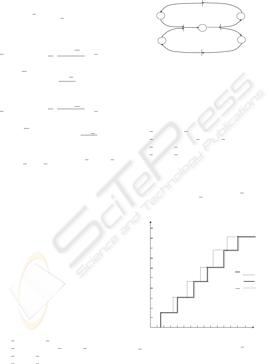
The evolution of the counter n
2
(t) is depicted in
figure 3 and is such that n
2
(t) ≤ n
2
(t) ≤
n
2
(t).
2
4
6
8
1 0
1 2
1 4
1 6
1 8
2 0
0
4 8 1 2 1 6
2 0
2 4 2 8
T i m e ( t )
E v e n t
n 2
n 2
n 2
Figure 3: The evolution of the counter variables n
2
, n
2
and
n
2
.
PERFORMANCE ANALYSIS OF TIMED EVENT GRAPHS WITH MULTIPLIERS USING (Min, +) ALGEBRA
19

4 PERFORMANCE EVALUATION
4.1 Elements of performance
evaluation for TEG
We recall main results characterizing an ordinary
TEG’s modelled in the dioid Z
min
(Baccelli et al.,
1992), (Gaubert, 1992).
Definition 2 (Irreducible matrix) A matrix A is
said irreducible if for any pair (i,j), there is an inte-
ger m such that (A
m
)
ij
6= ε.
Theorem 1 Let A be a square matrix with coefficient
in Z
min
. The following assertions are equivalent:
• Matrix A is irreducible,
• The TEG associated with matrix A is strongly con-
nected.
One calls eigenvalue and eigenvector of a matrix A
with coefficients in Z
min
, the scalar λ and the vector
υ such as:
A ⊗ υ = λ ⊗ υ.
When the initial vector x(0) of matrix equation (3) is
equal to an eigenvector of matrix A, the TEG reaches
a periodic regime from the initial state.
Theorem 2 Let A be a square matrix with coeffi-
cients in Z
min
. If A is irreducible, or equivalently, if
the associated TEG is strongly connected, then there
is a single eigenvalue denoted λ. The eigenvalue can
be calculated in the following way:
λ =
n
M
j=1
(
n
M
i=1
(A
j
)
ii
)
1
j
. (8)
Regarding the TEG, λ corresponds to the firing
rate identical for each transition. This eigenvalue λ
can be directly deduced from the TEG by
λ = min
c∈ C
M(c)
T (c)
, (9)
where:
• C is the set of elementary circuits of the TEG .
• T(c) is the sum of holding times in circuit c.
• M(c) is the number of tokens in circuit c.
It is possible that several eigenvectors can be associ-
ated with the only eigenvalue of an irreductible ma-
trix.
Definition 3 Let A be an irreducible matrix of eigen-
value λ. One defines the matrix denoted A
λ
by
A
λ
= λ
−1
⊗ A.
Theorem 3 (Gondran and Minoux, 1977) Let A be
an irreducible matrix of eigenvalue λ. The j-th col-
umn of the matrix A
+
λ
, denoted (A
+
λ
)
j
, is an eigen-
vector of A if it satisfies the following equality:
(A
+
λ
)
j
= A
λ
⊗ (A
+
λ
)
j
. (10)
4.2 Elements of performance
evaluation for TEGM’s
In the case of TEGM’s, the firing rate, denoted λ
m
q
,
is not identical for all transitions. It is defined as fol-
lows:
λ
m
q
=
θ
q
T C
m
, (11)
where θ
q
is the component of the T-semiflow associ-
ated with transition q, and T C
m
is average the cycle
time of the TEGM.
The average cycle time of a TEGM can be defined
as follows :
Definition 4 (Sauer, 2003)
The average cycle time, TC
m
, of a TEGM is the aver-
age time to fire once the T-semiflow under the earliest
firing rule (i.e., transitions are fired as soon as possi-
ble) from the initial marking.
The firing rate λ
m
q
of a linearizable TEGM can be
calculated from the (min, +) linear model by:
λ
m
q
= θ
q
λ (12)
where λ is the eigenvalue of the equivalent (min,+)
linear model. This result is a direct consequence of
the linearization proprety.
In the case where we have an approximate lin-
earization, we obtain
λ
m
q
≤ λ
m
q
≤
λ
m
q
,
where
λ
m
q
(resp., λ
m
q
) is the firing rate of the
transition q obtained by using the upper (resp., lower)
approximated linear model of the TEGM.
When components of the eigenvector, associated
with the TEG obtained by linearization, are integer
values, the initial conditions vector of TEGM, de-
noted υ
m
(which allow to reach the periodic regime
from the initial state) can be deduced by:
υ
m
= (θ
1
x
1
(0), ..., θ
n
x
n
(0)) (13)
where x(0) is the eigenvector of the TEG.
ICINCO 2005 - SIGNAL PROCESSING, SYSTEMS MODELING AND CONTROL
20

Example 3 One determines the firing rate for each
transition of the TEGM of figure 1 from the (min, +)
linear model.
For M(0) = (6, 0, 0, 3, 0), the initial marking of
each place verifies the linearization condition. This
TEGM is linearizable.
Thanks to Eq.(8), the production rate of the TEG
obtained after linearization is equal to
1
5
. From
Eq.(12), we deduce the firing rate of each transition:
λ
m
1
=
2
5
, λ
m
2
=
3
5
, λ
m
3
=
3
5
, λ
m
4
=
1
5
.
Thanks to Eq.(11), we deduce that T C
m
= 5.
For initial marking M(0)=(6,0,0,4,0), we have two
linear approximated (min, +) models.
In the case where we add two tokens in the place
P4 in the TEGM, we obtain a TEG with λ is equal to
1
4
.
Thanks to Eq.(12), we deduce the firing rate of
each transition :
λ
m
1
=
3
4
,
λ
m
2
=
2
4
,
λ
m
3
=
2
4
,
λ
m
4
=
1
4
.
Thanks to equation (11), we deduce
T C
m
= 4.
In the case where we remove one token in the place
P4, we obtain a TEG with λ is equal to
1
5
.
Thanks to Eq.(12), we deduce the firing rate of
each transition :
λ
m
1
=
3
5
, λ
m
2
=
2
5
, λ
m
3
=
2
5
, λ
m
4
=
1
5
.
Thanks to Eq.(11), we deduce T C
m
= 5.
Finally, for M(0)=(6,0,0,4,0), we obtain:
4 ≤ T C
m
≤ 5
3
5
≤ λ
m
1
≤
3
4
,
2
5
≤ λ
m
2
≤
2
4
,
2
5
≤ λ
m
3
≤
2
4
,
1
5
≤ λ
m
4
≤
1
4
.
5 CONCLUSION
In order to evaluate the performances of a TEGM
from an equivalent TEG, a technique of linearization
has been proposed in (min,+) algebra. According to
initial marking, a linearization condition was stated.
The performance analysis of a linearizable TEGM,
such as cycle times, is deduced directly from the ob-
tained linear model.
REFERENCES
Baccelli, F., Cohen, G., Olsder, G., and Quadrat, J.-P.
(1992). Synchronization and Linearity: An Algebra
for Discrete Event Systems. Wiley.
Chao, D., Zhou, M., and Wang, D. (1993). Multiple
Weighted Marked Graphs. In IFAC 12th Triennial
World Congress, pages ”371–374”, Sydney, Australie.
Cohen, G., Gaubert, S., and Quadrat, J.-P. (1998). Timed-
event graphs with multipliers and homogeneous min-
plus systems. IEEE TAC, 43(9):1296–1302.
Gaubert, S. (1992). Th
´
eorie des syst
`
emes lin
´
eaires dans les
dio
¨
ıdes. Th
`
ese de doctorat, Ecole des mines de Paris.
Gondran, M. and Minoux, M. (1977). Valeurs propres et
vecteurs propres dans les dio
¨
ıdes et leur interpr
´
etation
en th
`
eorie des graphes. volume 2, pages 25–41. EDF,
Bullettin de la Direction des Etudes et Recherche, Se-
rie C, Math
´
ematiques informatique.
Hamaci, S., Boimond, J.-L., and Lahaye, S. (2004). On the
Linearizability of Discrete Timed Event Graphs with
Multipliers Using (min,+) Algebra. In WODES, pages
367–372.
Munier, A. (1993). R
´
egime asymptotique optimal d’un
graphe d’
´
ev
´
enements temporis
´
e g
´
en
´
eralis
´
e : applica-
tion
`
a un probl
`
eme d’assemblage. In RAIPO-APII,
volume 27(5), pages 487–513.
Murata, T. (1989). Petri Nets: Properties, Analysis and Ap-
plications. In Proceedings of the IEEE, volume 77(4),
pages 541–580.
Nakamura, M. and Silva, M. (1999). Cycle Time Compu-
tation in Deterministically Timed Weighted Marked
Graphs. In IEEE-ETFA, pages 1037–1046.
Sauer, N. (2003). Marking Optimization of Weighted
Marked Graphs. Journal of Discrte Event Dynamic
Systems, 13:245–262.
Trouillet, B., Benasser, A., and Gentina, J.-C. (2002). On
the Modeling of the Dynamical Behavior of Weighted
T-Systems. In APII-JESA, volume 36(7), pages 931–
944.
PERFORMANCE ANALYSIS OF TIMED EVENT GRAPHS WITH MULTIPLIERS USING (Min, +) ALGEBRA
21
