
TRACKING-CONTROL INVESTIGATION OF TWO X4-FLYERS
K. M. Zemalache, L. Beji and H. Maaref
Universit
´
e d’Evry - CNRS FRE 2494
Laboratoire Syst
`
emes Complexes (LSC)
40 rue du Pelvoux,91020 Evry Cedex, France
Keywords:
X4-flyer, dynamical systems, backstepping control, tracking control.
Abstract:
Two models of mini-flying robots with four rotors called X4-flyer presented and studied for the stabilization.
Both cases with and without motion planning are proposed in this paper. The first is called inertial model with
axes orientation and the second is called the inertial model without axes orientation. The control algorithm of
the X4-flyer is based on the Lyapunov method and obtained using the backstepping techniques. This enabled
to stabilize the engine in hovering and to generate its trajectory. The system behavior using the proposed
control law is described through numerical simulations.
1 INTRODUCTION
The automatic control of flying machines has at-
tracted the attention of many researches in the past
few years. Generally, the control strategies are based
on simplified models which have both a minimum
number of states and a minimum number of input.
These reduced models should retain the main features
that must be considered when designing control laws
for real aerial vehicles. The rotorcraft is one the most
complex flying machines. Its complexity is due to
the versatility and manoeuvrability to perform many
types of tasks (Castillo et al., 2004). Very little atten-
tion has been done on the development of aerial ro-
botic platforms (Altug, 2003) (Altug et al., 2003) (Al-
tug et al., 2002) (Hamel et al., 2002) (Zhang, 2000).
Such platforms have considerable commercial poten-
tial for surveillance and inspection roles in dangerous
environments.
Modelling and controlling aerial vehicles (blimps,
mini rotorcraft) are the principal preoccupation of our
laboratory (LSC). In this topic, a mini-UAV is de-
velopped by the LSC-group taking into account in-
dustrial constraints. The aerial flying engine could
not exceed 2kg in mass, a wingspan of 50cm with
a 30mn flying-time (see figure 1). Within this optic,
it can be held that our system belongs to a family of
mini-UAV. It is an autonomous hovering system, ca-
pable of vertical takeoff, landing, lateral motion and
quasi-stationary (hover or near hover) flight condi-
tions. Compared to helicopters (Altug, 2003) (Altug
et al., 2003) (Altug et al., 2002), the four rotors ro-
torcraft called X4-flyer has some advantages (Hamel
et al., 2002) (Pound et al., 2002): given that two mo-
tors rotate counter clockwise while the other two ro-
tate clockwise, gyroscopic effects and aerodynamic
torques tend, in trimmed flight, to cancel. An X4-flyer
operates as an omnidirectional UAV. Vertical motion
is controlled by collectively increasing or decreasing
the power for all motors. Lateral motion, in x direc-
tion or in y direction, is achieved by differentially
controlling the motors generating a pitching/rolling
motion of the airframe that inclines the collective
thrust (producing horizontal forces) and leads to lat-
eral accelerations.
Several recent work was completed for the design
and control in pilot-less aerial vehicles domain such
that Quadrotor (Altug, 2003) (Altug et al., 2003) (Al-
tug et al., 2002), X4-flyer (Hamel et al., 2002), mesi-
copter (Kroo and Printz, ) and hoverbot (Borenstein,
). Also, related models for controlling the VTOL
aircraft are studied by Hauser and al (Hauser et al.,
1992). A model for the dynamic and configuration
stabilization of quasi-stationary flight conditions of a
four rotors vertical take-off and landing (VTOL) was
studied by Hamel (Hamel et al., 2002) where the dy-
namic motor effects are incorporating and a bound of
perturbing errors was obtained for the coupled sys-
tem. The stabilization problem of a four rotors rotor-
craft is also studied and tested by Castillo (Castillo
16
M. Zemalache K., Beji L. and Maaref H. (2005).
TRACKING-CONTROL INVESTIGATION OF TWO X4-FLYERS.
In Proceedings of the Second International Conference on Informatics in Control, Automation and Robotics - Robotics and Automation, pages 16-23
DOI: 10.5220/0001157600160023
Copyright
c
SciTePress
et al., 2004) where the nested saturation algorithm is
used and application of the theory of flat systems by
Beji et al (Beji et al., 2004).
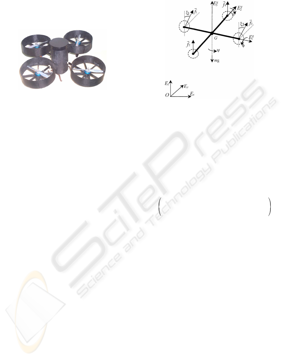
Figure 1: Conceptual form of the four rotors rotorcraft.
In this paper, the backstepping controllers and mo-
tion planning are combined to stabilize the helicopter
by using the point to point steering stabilization. Af-
ter having presented the study of modeling and the
description of the configuration in the second section.
Third section describes the dynamics of the system
which treats the two models with and without axes
orientation. Backstepping controllers is described for
two models of the X4-flyer in the fourth section. A
strategy to solve the tracking problem through point
to point steering is shown in the fifth section. In the
sixth section simulation results are introduced for two
models. Finally, conclusion and future work are given
in the last section.
2 CONFIGURATION
DESCRIPTION AND
MODELLING
Unlike regular helicopters that have variable pitch an-
gles, an engine has fixed pitch angle rotors and the
rotor speeds are controlled to produce the desired lift
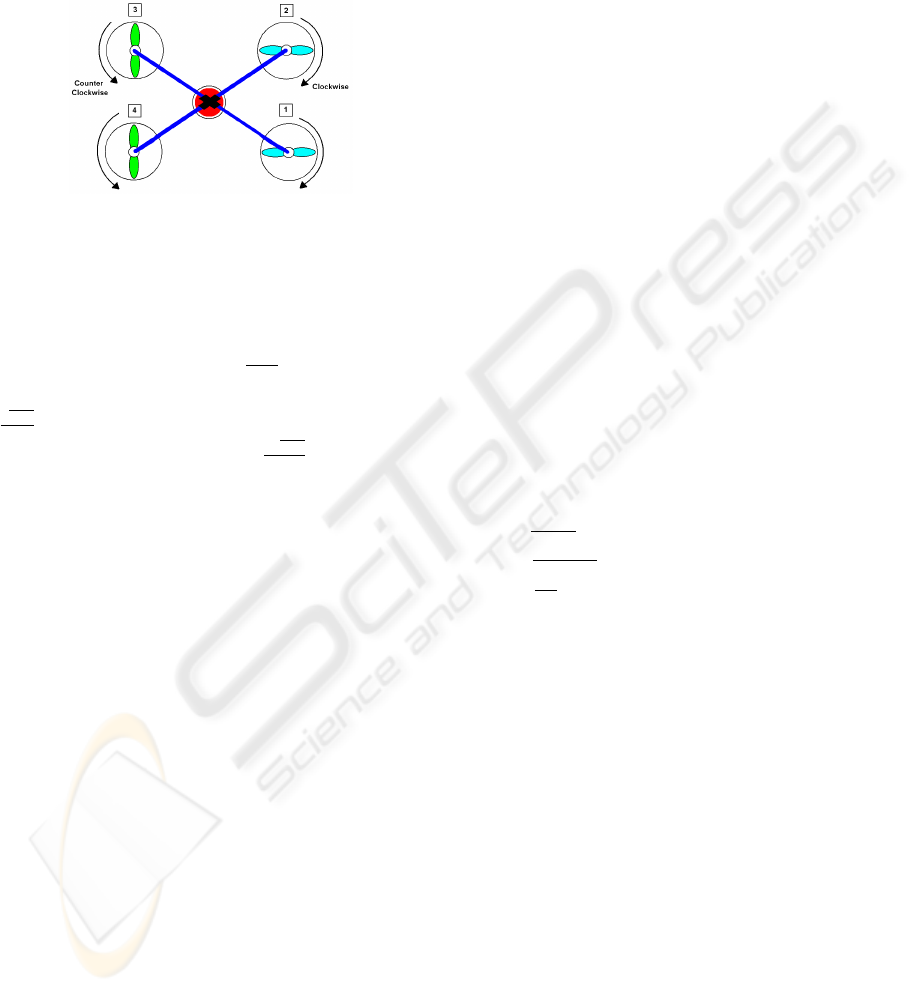
forces. Basic motions of the four rotors rotorcraft
can described using the figure 2. Vertical motion is
controlled by collectively increasing or decreasing the
power for all motors. Lateral motion, in x direction or
in y direction, is not achieved by differentially con-
trolling the motors generating a pitching/rolling mo-
tion of the airframe that inclines the collective thrust
(producing horizontal forces) and leads to lateral ac-
celerations (case of the X4-flyer). But, two engines
of direction are used to permute between the x and y
motion.
We consider a local reference airframe ℜ
G
=
{G, E
g
1
, E
g
2
, E
g
3
} attached to the mass center G of the
vehicle. The mass center is located at the intersec-
tion of the two rigid bars, each of which supports two
motors. Equipments (controller cartes, sensors, etc.)
Figure 2: 3D X4-flyer model.
onboard are placed not far from G. The inertial frame
is denoted by ℜ
O
= {O, E
x
, E
y
, E
z
}. A body fixed
frame is assumed to be at the center of gravity of the
X4-flyer, where the z axis is pointing upwards. This
body axis is related to the inertial frame by a position
vector (x, y, z) and 3 Euler angles (θ, φ, ψ) represent-
ing pitch, roll and yaw respectively. A Euler angle
representation given in (1) has been chosen.
R =
C
ψ
C
θ
C
θ
S
ψ
−S
θ
S
φ
C
ψ
S
θ
− S
ψ
C
φ
S
θ
S
ψ
S
φ
+ C
ψ
C
φ
C
θ
S
φ
S
θ
C
ψ
C
φ
+ S
ψ
S
φ
C
φ
S
θ
S
ψ
− C
ψ
S
φ
C
θ
C
φ
(1)
Where C
θ
and S
θ
represent cos θ and sin θ repec-
tively.
Each rotor produces moments as well as vertical
forces. These moments have been experimentally ob-
served to be linearly dependent on the forces for low
speeds. There are four/five input forces and six out-
put states (x, y, z, θ, φ, ψ) therefore the X4-flyer is an
under-actuated system. The rotation direction of two
of the rotors are clockwise while the other two are
counterclockwise, in order to balance the moments
and produce yaw motions as needed.
In the present work, two X4-flyer models are pre-
sented, the first is called the inertial model with axes
orientation, the second one is the inertial model with-
out axes orientation. For the model without axes ori-
entation, the rotors 2 and 4 are actuated in clock-
wise direction, the remain rotors, the rotors 1 and 3
are in the contrary actuated in the inverse direction
in order to guarantee total balance in yaw (figure 4).
The main feature of the presented X4-flyer (called the
XSF) in comparison with the existing quadrirotors, is
the swiveling of the actuators supports 1 and 3 around
the axis of pitching (angles ξ
1
and ξ
3
). This swiveling
ensures either the horizontal rectilinear motion or the
TRACKING-CONTROL INVESTIGATION OF TWO X4-FLYERS
17
rotational movement around the yaw axis or a combi-
nation of these two movements which gives the turn
(see the figure 3), as well as the direction of rotation
of the rotors implies that rotors 1 and 2 turn clockwise
and rotors 3 and 4 turn in the contrary direction of the
needles of a watch.
Figure 3: Rotor rotations with canceled yaw motions.
3 MOTION DYNAMIC
We consider the translation motion of ℜ
G
with re-
spect to (wrt) ℜ
O
. The position of the center of
mass wrt ℜ
O
is defined by
OG = (x y z)
T
, its
time derivative gives the velocity wrt to ℜ
O
such that
d
OG
dt
= ( ˙x ˙y ˙z)
T
, while the second time derivative
permits to get the acceleration
d
2
OG
dt
2
= (¨x ¨y ¨z)
T
.
In the following, the model with axes orientation is
described, then the model without axes orientation is
given.
3.1 Dynamic Motion of the Model
with Axes Orientation
Currently, the model is a simplified one’s. The con-
straints and the gyroscopic torques are neglected. The
aim is to control the engine vertically (z) axis and hor-
izontally according to x and y axis. The dynamics of
the vehicle, represented on figure 2, is modelled by
the system of equations (2), (Beji et al., 2005).
m¨x = S
ψ
C
θ
u
2
− S
θ
u
3
m¨y = (S
θ
S
ψ
S
φ
+ C
ψ
C
φ
) u
2
+ C
θ
S
φ
u
3
m¨z = (S
θ
S
ψ
C
φ
− C
ψ
C
φ
) u
2
+ C
θ
C
φ
u
3
− mg
(2)
Where m is the total mass of the vehicle. The vec-
tor u
2
and u
3
combines the principal non conservative
forces applied to the engine airframe including forces
generated by the motors and drag terms. Drag forces
and gyroscopic due to motors effects will be not con-
sidered in this work. The lift (collective) force u
3
and
the direction input u
2
are such that
0
u
2
u
3
!
= f
1
´e
1
+ f
2
e
2
+ f
3
´e
3
+ f
4
e
4
(3)
with f
i
= k
i
ω
2
i
, k
i
> 0 is a given constant and ω
i
is the angular speed resulting of motor i. Let
´e
1
=
0
S
ξ
1
C
ξ
1
!
ℜ
G
; ´e
3
=
0
S
ξ
3
C
ξ
3
!
ℜ
G
e
2
= e
4
=
0
0
1
!
ℜ
G
(4)
Then we deduce:
u
2
= f
1
S
ξ
1
+ f
3
S
ξ
3
u
3
= f
1
C
ξ
1
+ f
3
C
ξ
3
+ f
2
+ f
4
(5)
ξ
1
and ξ
3
are the two internal degree of freedom of
rotors 1 and 3, respectively. These variables are con-
trolled by dc-motors and bounded −20
o
≤ ξ
1
, ξ
3
≤
+20
o
. e
2
and e
4
are the unit vectors along E
g
3
which
imply that rotors 2 and 3 are identical of that of a clas-
sical Quadrotor (not directional).
3.2 Rotational Motion of the Model
with Axes Orientation
The rotational motion of the X4 bidirectional flyer
will be defined wrt to the local frame but ex-
pressed in the inertial frame. According to Classi-
cal Mechanics, and knowing the inertia matrix I
G
=
diag (I
xx
, I
yy
, I
zz
) at the centre of the mass.
¨
θ =
1
I
xx
C
φ
(τ
θ
+ I
xx
S
φ
˙
φ
˙
θ)
¨
φ =
1
I
yy
C
θ
C
φ
(τ
φ
+ I
yy
S
φ
C
θ
φ˙
2
+ I
yy
S
θ
C
φ
˙
θ
˙
φ)
¨
ψ =
τ
ψ
I
zz
(6)
With the three inputs in torque
τ
θ
= l (f
2
− f
4
)
τ
φ
= l (f
1
C
ξ
1
− f
3
C
ξ
3
)
τ
ψ
= l (f
1
S
ξ
1
− f
3
S
ξ
3
)
(7)
where l is the distance from G to the rotor i. The
equality from (6) is ensured, meaning that
¨η = Π
G
(η)
−1
[τ −
˙
Π
G
(η) ˙η] (8)
With τ = (τ
θ
, τ
φ
, τ
ψ
)
T
as an auxiliary inputs.
And
Π
G
(η) =
I
xx
C
φ
0 0
0 I
yy
C
φ
C
θ
0
0 0 I
zz
!
(9)
As a first step, the model given above can be
input/output linearized by the following decoupling
feedback laws
τ
θ
= −I
xx
S
φ
˙
φ
˙
θ + I
xx
C
φ
˜τ
θ
τ
φ
= −I
yy
S
φ
C
θ
˙
φ
2
− I
yy
S
θ
C
φ
˙
θ
˙
φ + I
yy
C
θ
C
φ
˜τ
φ
τ
ψ
= I
zz
˜τ
ψ
(10)
ICINCO 2005 - ROBOTICS AND AUTOMATION
18
and the decoupled dynamic model of rotation can
be written as
¨η = ˜τ (11)
with ˜τ = (˜τ
θ
˜τ
φ
˜τ
ψ
)
T
Using the system of equations (2) and (11), the dy-
namic of the system is defined by
m¨x = S
ψ
C
θ
u
2
− S
θ
u
3
m¨y = (S
θ
S
ψ
S
φ
+ C
ψ
C
φ
) u
2
+ C
θ
S
φ
u
3
m¨z = (S
θ
S
ψ
C
φ
− C
ψ
C
φ
) u
2
+ C
θ
C
φ
u
3
− mg
¨
θ = ˜τ
θ
;
¨
φ = ˜τ
φ
;
¨
ψ = ˜τ
ψ
(12)
3.3 Dynamic Motion of the Model
without Axes Orientation
We follows the same steps as the model with axes ori-
entation and finally we finds for the dynamics of the
X4-flyer without the axes orientation:
m¨x = −S
θ
u
3
m¨y = C
θ
S
φ
u
3
m¨z = C
θ
C
φ
u
3
− mg
(13)
3.4 Rotational Motion of the Model
without Axes Orientation
The three inputs in torque are given by:
τ
θ
= l (f
2
− f
4
)
τ
φ
= l (f
1
− f
3
)
τ
ψ
= lk (f
1
− f
2
+ f
3
− f
4
)
(14)
The vertical controller is: u
3
= f
1
+ f
3
+ f
2
+ f
4
Using the translational and rotational motions (13)
and (14), equations of the dynamic are detailed by
m¨x = −S
θ
u
3
m¨y = C
θ
S
φ
u
3
m¨z = C
θ
C
φ
u
3
− mg
¨
θ = ˜τ
θ
;
¨
φ = ˜τ
φ
;
¨
ψ = ˜τ
ψ
(15)
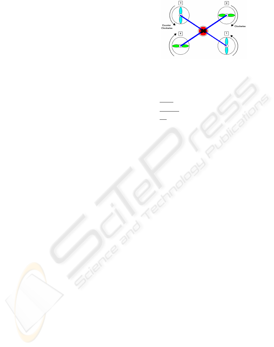
Remark: As shown in the system (2), the three inputs
torque see the equation (7), the yaw τ
ψ
is equal to
zero if we take ξ
1
= ξ
3
= 0. Then, with the proposed
sense of rotations (see figure 3), we can not generate
yaw motions if rotors 1 and 3 are not oriented. With
ξ
1
= ξ
3
= 0, to obtain yaw motions, the rotor sense
of rotations is identical of that of the Quadrotor.
Then rotors 1 and 3 are with the same sense of rota-
tions, while rotors 2 and 4 are in opposite sense (see
figure 4).
With or without axes orientation, the rotational part
can be easily linearized with static feedback control
laws. Then, we get
¨
θ = u
4
¨
φ = u
5
¨
ψ = u
6
(16)
Figure 4: Rotor rotations with yaw motions.
with
u
4
=
1
I
xx
C
φ
(τ
θ
+ I
xx
S
φ
˙
φ
˙
θ)
u
5
=
1
I
yy
C
θ
C
φ
(τ
φ
+ I
yy
S
φ
C
θ
˙
φ
2
+ I
yy
S
θ
C
φ
˙
θ
˙
φ)
u
6
=
1
I
zz
τ
ψ
(17)
4 BACKSTEPPING BASED
CONTROLLER
Backstepping controllers are especially useful when
some states are controlled through other states. As
it was observed in the previous section, in order to
control the x and y motion of the X4-flyer, tilt an-
gles need to be controlled. Therefore a backstepping
controller has been developed in this section. Similar
ideas of using backstepping with visual serving have
been developed for a traditional helicopter by Hamel
and Mahony (Hamel and Mahony, 2000). As well as
the backstepping controllers was applied for Quadro-
tor by Altug et al (Altug, 2003) (Altug et al., 2003)
(Altug et al., 2002).
4.1 ”Backstepping” Application to
the Model without Axes
Orientation
4.1.1 Altitude and yaw control
The altitude and the yaw on the other hand, can be
controlled by a PD controller. With through the equa-
tion of the following movement (z).
m¨z = C
θ
C
φ
u
3
− mg (18)
The control of the vertical position (altitude) can be
obtained considering the following control input
u
3
= m
g + ¨z
r
− k
1
z
( ˙z − ˙z
r
) − k
2
z
(z − z
r
)
(19)
with
¨z = ¨z
r
− k
1
z
( ˙z − ˙z
r
) − k
2
z
(z − z
r
) (20)
TRACKING-CONTROL INVESTIGATION OF TWO X4-FLYERS
19

z
r
is the desired altitude. The yaw attitude can be
stabilized to a desired value with the following track-
ing feedback control
u
6
=
¨
ψ
r
− k
1
ψ
(
˙
ψ −
˙
ψ
r
) − k
2
ψ
(ψ − ψ
r
) (21)
where k
1
z
, k
2
z
, k
1
ψ
, k
2
ψ
are the coefficients of stable
polynomial.
4.1.2 Roll control (φ, y)
First we notice that motion in the y direction can
be controlled through the changes of the roll angle.
These variables are related by the cascade system
m¨y = C
θ
S
φ
u
3
¨
φ = u
5
(22)
This leads to a backstepping controller for y − φ
control given by
u
5
=
1
u
3
C
θ
C
φ
(5y + 10 ˙y + u
3
Θ
θ,φ
) (23)
where
Θ
θ,φ
=
9S
φ
C
θ
+ 4
˙
φC
φ
C
θ
−
˙
φ
2
S
φ
C
θ
−
2
˙
θS
φ
S
θ
+
˙
φ
˙
θC
φ
S
θ
−
˙
θ
˙
φC
φ
S
θ
+
˙
θ
2
S
φ
C
θ
(24)
4.1.3 Pitch control (θ, x)
To develop a controller for motion along the x axis,
similar analysis is needed. The equation of motion of
the X4-flyer on x is given as
m¨x = −S
θ
u
3
¨
θ = u
4
(25)
This leads to a backstepping controller for x − θ
control given by
u
4
=
1
u
3
C
θ
(−5x − 10 ˙x + u
3
Θ
θ
) (26)
where
Θ
θ
= 9S
θ
+ 4
˙
θC
θ
−
˙
θ
2
S
θ
(27)
4.2 Model with Axes Orientation
4.2.1 Control input for (z − y) motions
We propose to control motion along y and z direc-
tions through u
3
and u
2
, respectively. So we have the
proposition (28).
¨y
¨z
=
1
m
H
u
2
u
3
−
0
g
(28)
where
H =
S
ψ
S
θ
S
φ
+ C
ψ
C
φ
C
θ
S
φ
S
ψ
S
θ
C
φ
− C
ψ
S
φ
C
θ
C
φ
(29)
For the given conditions in ψ and θ , the 2 by 2
matrix (29) is invertible. Then a nonlinear decou-
pling feedback permits to write the following decou-
pled linear dynamics
¨y = ν
y
¨z = ν
z
(30)
Then we can deduce from (30) the linear controller
ν
y
= ¨y
r
− k
1
y
( ˙y − ˙y
r
) − k
2
r
(y − y
r
)
ν
z
= ¨z
r
− k
1
z
( ˙z − ˙z
r
) − k
2
z
(z − z
r
)
(31)
With the k
i
y
and k
i
z
are the coefficients of a polyno-
mial of Hurwitz
Proposition: Consider
(ψ, θ) ∈
i
−
π
2
,
π
2
h
(32)
with the controllers (33) and (34)
u
2
=
C
φ
C
ψ
(m¨y) −
S
φ
C
ψ
(m (¨z + g)) (33)
u
3
=
−S
ψ
S
θ
C
φ
+C
ψ
S
φ
C
θ
C
ψ
(m¨y) +
S
ψ
S
θ
S
φ
+C
ψ
C
φ
C
θ
C
ψ
(m (¨z + g))
(34)
The dynamic of y and z are linearly decoupled and
exponentially-asymptotically stable with the appro-
priate choice of the gain controller parameters.
4.2.2 Control input for the x motion
To control the movement along the x axis, the back-
stepping controller is used. The noted controller x −θ
is given by the equation (35):
m¨x = S
ψ
C
θ
u
2
− S
θ
u
3
¨
θ = u
4
(35)
One supposes it exists a time T
1
f
such that ∀t∈
h
T
0
, T
1
f
i
, u
3
> 0, then the dynamic of x is decou-
pled under the following controller
u
4
=
1
u
3
C
θ
+ u
2
S
θ
S
ψ
(−5x − 10 ˙x + u
3
Θ
θ
+ u
2
Θ
θ,ψ
)
(36)
where
Θ
θ
= 9S
θ
+ 4
˙
θC
θ
−
˙
θ
2
S
θ
(37)
and
Θ
θ,ψ
=
9S
ψ
C
θ
+ 4
˙
θC
ψ
C
θ
−
˙
ψ
2
S
ψ
C
θ
−
2
˙
ψS
ψ
S
θ
+
˙
ψ
˙
θC
ψ
S
θ
−
˙
θ
˙
ψC
ψ
S
θ
+
˙
θ
2
S
ψ
C
θ
(38)
ICINCO 2005 - ROBOTICS AND AUTOMATION
20
5 TRAJECTORY GENERATION
AND POINT TO POINT
STEERING
Due to the structure limit of the X4-flyer, motion can
be asserted only in straight line along the x, y and z
directions. In our case, that is sufficient to navigate in
a region. Otherwise, an other version of the engine is
under study by the group. The version flyer is to make
easy manoeuvres in corners with arc of circle. In the
following, we solve the tracking problem as point to
point steering one over a finite interval of time. Then
we take each ending point with its final time as a new
starting point.
0 2 4 6 8
0
5
10
15
z−ref (m)
time (s)
10 15 20 25
0
5
10
15
time (s)
x−ref (m)
20 25 30 35
0
5
10
15
y−ref (m)
time (s)
0
10
20
0
10
20
0
5
10
x−displacement
y−displacement
z−displacement
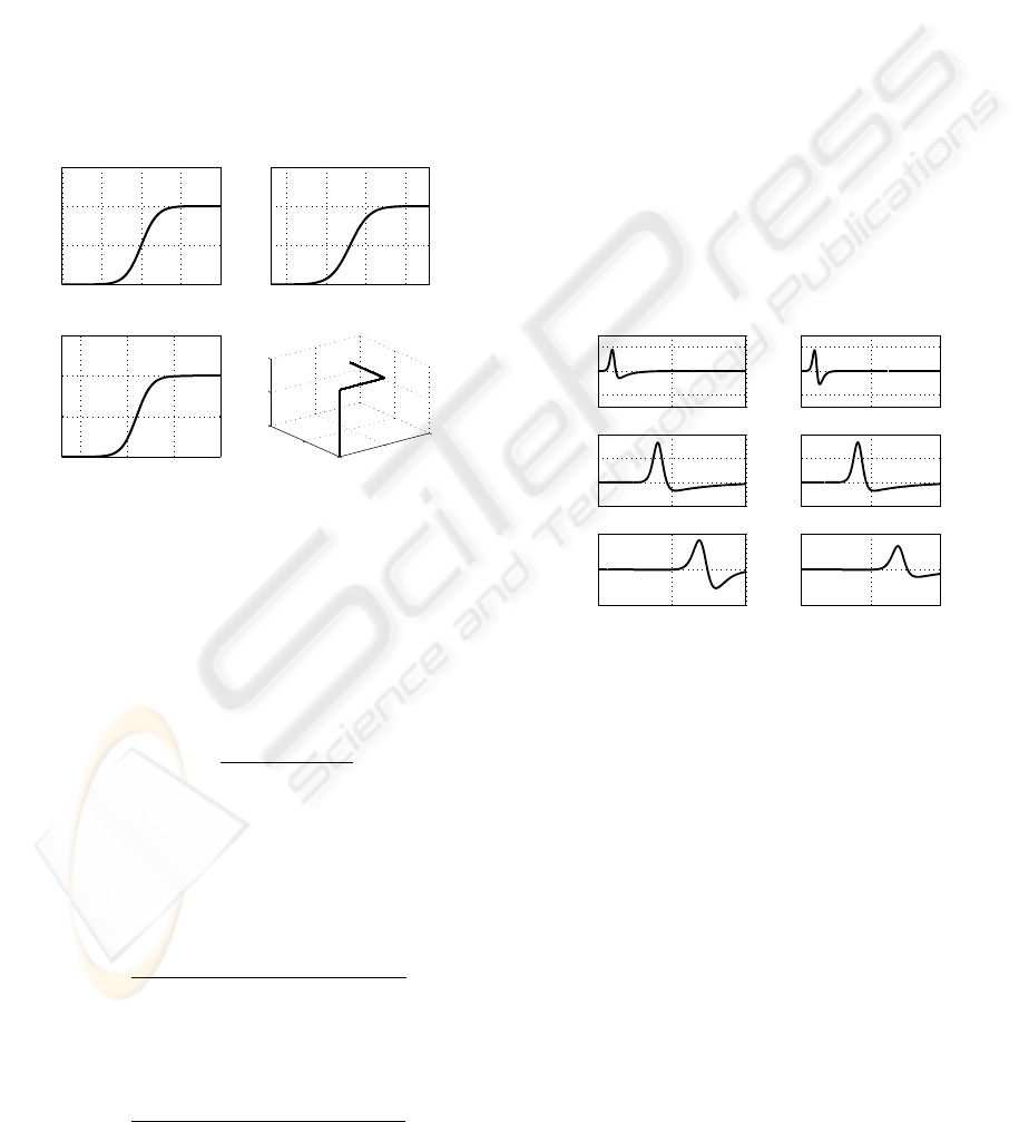
Figure 5: Motion planning with h
d
= 10m.
Figure 5 illustrate the reference trajectory along the
x, y and z directions. As we see, the X4-flyer will fly
in the z direction followed by the x − motion and the
y−motion. The reference trajectory is parameterized
as
z
r
(t) = h
d
t
5
t
5
+ (T
1
f
− t)
5
(39)
where h
d
is the desired altitude and (T
1
f
) the final
time. In order to solve the point to point steering con-
trol, the end point of the trajectory (39) can be adopted
as initial point to move along x, then we have
x
r
(t) = h
d
(t − T
1
f
)
5
(t − T
1
f
)
5
+ (T
2
f
− (t − T
1
f
))
5
(40)
As soon as for y
r
(t)
y
r
(t) = h
d
(t − T
2
f
)
5
(t − T
2
f
)
5
+ (T
3
f
− (t − T
2
f
))
5
(41)
The constraints to perform these trajectories are
such that
z
r
(0) = x
r
(T
1
f
) = y
r
(T
2
f
) = 0
z
r
(T
1
f
) = x
r
(T
2
f
) = y
r
(T
3
f
) = h
d
˙z
r
(0) = ˙x
r
(T
1
f
) = ˙y
r
(T
2
f
) = 0
˙z
r
(T
1
f
) = ˙x
r
(T
2
f
) = ˙y
r
(T
3
f
) = 0
¨z
r
(0) = ¨x
r
(T
1
f
) = ¨y
r
(T
2
f
) = 0
¨z
r
(T
1
f
) = ¨x
r
(T
2
f
) = ¨y
r
(T
3
f
) = 0
(42)
Minimizing the time of displacement implies that
the X4-flyer accelerates at the beginning and deceler-
ates at the arrival.
6 SIMULATION RESULTS
Two engine models were studied and controlled us-
ing the backstepping technique which (a) present the
model with axes orientation and (b) the model with-
out axes orientation.
0 20 40
−0.2
0
0.2
z−erreur (m)
0 20 40
−1
0
1
2
x−erreur (m)
0 20 40
−0.05
0
0.05
y−erreur (m)
0 20 40
−0.2
0
0.2
z−erreur (m)
0 20 40
−1
0
1
2
x−erreur (m)
0 20 40
−1
0
1
y−erreur (m)
time (s)
(a)
(b)
Figure 6: Displacement errors: (a) with axes orientation -
(b) without axes orientation.
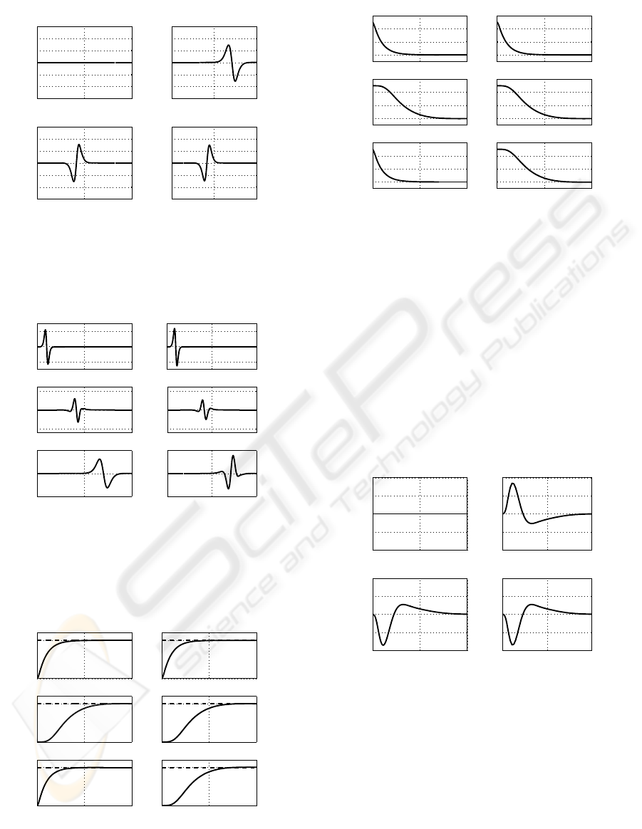
Figure 6 show displacement errors according to all
the directions for the models with and without axes
orientations. It is noticed that the error thus tends to
zero towards the desired positions.
Figure 7, we notices that the angles θ and φ control
the engine for displacements along the axes x and y.
These angles tend to zero value. It is also shown in
figure 8(a) that we can stabilize the system to make a
following movement by the swivelling of the engine
actuators 1 and 3.
According to the figure 8, which represent our ve-
hicle input, we remark that the input u
3
= mg at the
equilibrium state is always verified. The inputs u
2
,
u
4
and u
5
tend to zero after having carried out the de-
sired orientation of the vehicle. These Figure 8 also
show the effectiveness of the used controllers laws.
TRACKING-CONTROL INVESTIGATION OF TWO X4-FLYERS
21
0 20 40
−0.1
−0.05
0
0.05
0.1
angle phi (rad)
0 20 40
−0.2
−0.1
0
0.1
0.2
angle theta (rad)
(a)
(b)
0 20 40
−0.1
−0.05
0
0.05
0.1
angle phi (rad)
0 20 40
−0.2
−0.1
0
0.1
0.2
angle theta (rad)
time (s)
Figure 7: The pitch θ and the roll φ: (a) with axes orienta-
tion - (b) without axes orientation.
0 20 40
10
20
30
u3 (N)
0 20 40
−0.5
0
0.5
u4 (Nm)
0 20 40
−2
0
2
u2 (N)
0 20 40
10
20
30
u3 (N)
0 20 40
−0.5
0
0.5
u4 (Nm)
0 20 40
−0.1
0
0.1
u5 (Nm)
time (s)
(a)
(b)
Figure 8: Inputs u
2
, u
3
, u
4
and u
5
for the xyz displace-
ment: (a) with axes orientation - (b) without axes orienta-
tion.
0 5 10
0
5
z,z
r
(m)
0 5 10
0
5
x,x
r
(m)
0 5 10
0
5
y,y
r
(m)
0 5 10
0
5
z,z
r
(m)
0 5 10
0
5
x,x
r
(m)
0 5 10
0
5
y,y
r
(m)
time (s)
(a)
(b)
Figure 9: Without motion planning with h
d
= 5m: (a) with
axes orientation - (b) without axes orientation.
0 5 10
0
2
4
6
z−erreur (m)
0 5 10
0
2
4
6
x−erreur (m)
0 5 10
0
2
4
6
y−erreur (m)
0 5 10
0
2
4
6
z−erreur (m)
0 5 10
0
2
4
6
x−erreur (m)
0 5 10
0
2
4
6
y−erreur (m)
time (s)
(a)
(b)
Figure 10: Tracking errors without motion planning (z
r
=
x
r
= y
r
= 5m): (a) with axes orientation - (b) without
axes orientation.
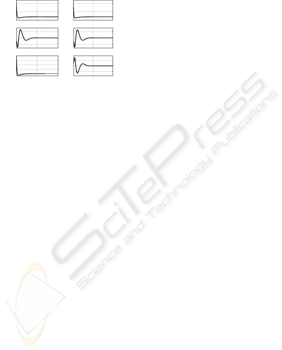
Figures 9,10,11 and 12, show the system without
motion planning. Motion in different directions z, x
and y is also tested and shown by figure 9. In addition
we show that the behavior of errors, given by figure
10 is verified. At the equilibrium, attitudes of θ and φ
are equal to zero (figure 11).
Without motion planning, the amplitude of controllers
is important (figure 12) and a maximum of energy is
asserted which is requested for flying vehicles.
0 5 10
−0.2
−0.1
0
0.1
0.2
angle phi (rad)
0 5 10
−0.2
−0.1
0
0.1
0.2
angle theta (rad)
(a)
(b)
0 5 10
−0.2
−0.1
0
0.1
0.2
angle phi (rad)
0 5 10
−0.2
−0.1
0
0.1
0.2
angle theta (rad)
time (s)
Figure 11: The pitch θ and the roll φ for the vehicle without
motion planning: (a) with axes orientation - (b) without axes
orientation.
7 CONCLUSION
The study of the stabilization with and without a pre-
defined trajectory of the mini-flying robot with four
rotors (X4-flyer) was discussed in this paper. The
importance of the trajectory generation and its con-
sequences with respect to amplitude of the used con-
troller, was highlited. With the proposed motion plan-
ICINCO 2005 - ROBOTICS AND AUTOMATION
22
0 5 10
0
50
100
u3 (N)
0 5 10
−0.5
0
0.5
u4 (Nm)
0 5 10
0
20
40
60
80
u2 (N)
0 5 10
0
50
100
u3 (N)
0 5 10
−0.5
0
0.5
u4 (Nm)
0 5 10
−0.5
0
0.5
u5 (Nm)
time (s)
(a)
(b)
Figure 12: Inputs u
2
, u
3
, u
4
and u
5
for the vehicle without
motion planning: (a) with axes orientation - (b) without axes
orientation.
ning, actuator saturations can be overcomed. Con-
sequently, economy in energy of batteries can be as-
serted during the fly. The backstepping technique was
successfully applied and enabled us to design control
algorithms ensuring the vehicle displacement from an
initial position to a desired position. The backstep-
ping approach used requires the well knowledge of
the system model and parameters. Future work is
to develop the fuzzy controller based algorithm (does
not require the good knowledge of the model) (Maaref
and Barret, 2001) and to make the comparison of both
controllers. A realization of a control system based on
engine sensors information is envisaged.
REFERENCES
Altug, E. (2003). Vision based control of unmanned aerial
vehicles with applications to an autonomous four ro-
tor helicopter, quadrotor. PhD thesis, faculties of the
university of Pennsylvania.
Altug, E., Ostrowski, J. P., and Mahony, R. (2002). Control
of a quadrotor helicopter using visual feedback. In
Proceeding of the IEEE International Conference on
Robotics and Automation, Washington D.C.
Altug, E., Ostrowski, J. P., and Taylor, C. (2003). Quadrotor
control using dual visual feedback. In Proceeding of
the IEEE International Conference on Robotics and
Automation, Taipei, Taiwan.
Beji, L., Abichou, A., and Slim, R. (2004). Stabilization
with motion planning of a four rotor mini-rotorcraft
for terrain missions. International Conference on Sys-
tems Design and Application, ISDA, Budapest, Hun-
gary.
Beji, L., Abichou, A., and Zemalache, K. M. (2005).
Smooth control of an x4 bidirectional rotors flying ro-
bots. Fifth International Workshop on Robot Motion
and Control, Dymaczewo, Poland.
Borenstein, J. Hoverbot project. University of Michi-
gin, www-personal.engin.umich.edu/ johannb/ Hover-
bot.htm.
Castillo, P., Dzul, A., and Lozano, R. (2004). Real-time sta-
bilization and tracking of a four rotor mini-rotorcraft.
IEEE Transactions on control Systems Technology.
Hamel, T. and Mahony, R. (2000). Visual serving of a class
of under-actuated dynamic rigid-body systems. Pro-
ceeding of the 39th IEEE Conference on decision and
control.
Hamel, T., Mahony, R., Lozano, R., and Ostrowski, J. P.
(2002). Dynamic modelling and configuration stabi-
lization for an x4-flyer. in IFAC 15th World Congress
on Automatic Control, Barcelona, Spain.
Hauser, J., Sastry, S., and Meyer, G. (1992). Nonlinear con-
trol design for slightly non-minimum phase systems:
Application to v/stol aircraft. Automatica.
Kroo, I. and Printz, F. Mesicopter project. Stanford Univer-
sity, http://aero.stanford.edu/ Mesicopter.
Maaref, H. and Barret, C. (2001). Progressive optimiza-
tion of a fuzzy inference system. IFSA-NAFIPS’2001,
Vancouver.
Pound, P., Mahony, R., Hynes, P., and Roberts, J. (2002).
Design of a four rotor aerial robot. Proceeding of
the Australasian Conference on Robotics and Automa-
tion, Auckland.
Zhang, H. (2000). Motion control for dynamic mobile ro-
bots. PhD thesis, faculties of the university of Penn-
sylvania.
TRACKING-CONTROL INVESTIGATION OF TWO X4-FLYERS
23
