
SETTLING-TIME IMPROVEMENT IN GLOBAL
CONVERGENCE LAGRANGIAN NETWORKS
Acho L.
Centro de Investigación y Desarrollo de Tecnología Digital del IPN (CITEDI-IPN)
CITEDI-IPN, 2498 Roll Dr. #757, Otay Mesa, San Diego CA, 92154, USA
Keywords: Lagrangian Networks, Global Convergence, Convex Optimization, Lyapunov Theory.
Abstract: In this brief, a modification of Lagrangian networks given in (Xia Y., 2003) is presented. This modification
improves the settling time of the convergence of Lagrangian networks to a stationary point; which is the
optimal solution to the nonlinear convex programming problem with linear equality constraints. This is
important because, in many real-time applications where Lagrangian networks are used to find an optimal
solution, such as in signal and image processing, this settling time is interpreted as the processing time.
Simulation results applied to a quadratic optimization problem show that settling time is improved from
about to 2000 to 20 seconds. Lyapunov theory was used to obtain our main result.
1 INTRODUCTION
Roughly speaking, a Lagrangian network is a
dynamical system used to find the optimal solution
to a nonlinear convex programming problem with
linear equality constraints (for more details, see (Xia
Y., 2003)). This dynamical system has simple
structure and its complexity for implementation is
low (Xia Y., 2003). Global convergence of a
Lagrangian network has been analyzed in (Xia Y.,
2003) and stated that it has not been studied before
(Xia Y., 2003). So, the convergence (in time) of the
solution of the Lagrangian networks to an
equilibrium point (or stationary point), which, under
some conditions, corresponds to the unique optimal
solution to the nonlinear convex programming
problem, is an important issue. In this short paper,
we present how to modify it to improve the settling
time convergence. Engineering applications in real-
time of Lagrangian networks, and important
references about it, are cited in (Xia Y., 2003). We
developed simulation experiments applied to a
quadratic optimization problem to show that the
settling time could be improved from about to 2000
to 20 seconds. Lyapunov theory is employed to
prove our main result.
2 CONVEX OPTIMIZATION
PROBLEM USING
LAGRANGIAN NETWORKS
Consider the following non-linear convex
programming problem with equality constraints (Xia
Y., 2003):
Minimize f(x) subject to Ax=b (1)
where f(x) is a smooth and strictly convex function,
nm
R
A
×
∈
, and . Remember that a
functional
is strictly convex function in
m
Rb ∈
RRf
n
→:
n
R
X
⊂
if, for all x,y
∈
X and
10 <<
α
, we have
that for all
y
x
≠
:
).()1()())1(( yfxfyxf
α
α
α
α
−+
<
−
+
(2)
Consider the next Lagrangian function:
)()(),( bAxyxfyxL
T
−−=
, (3)
where is referred as the Lagrangian
multiplier. is a solution to (1) if and only if there
exists such that ( , ) satisfies the
m
Ry ∈
∗
x
m
Ry ∈
*
∗
x
∗
y
315
L. A. (2005).
SETTLING-TIME IMPROVEMENT IN GLOBAL CONVERGENCE LAGRANGIAN NETWORKS.
In Proceedings of the Second International Conference on Informatics in Control, Automation and Robotics, pages 315-318
Copyright
c
SciTePress

following Lagrangian conditions (see (Xia Y.,
2003)):
0)(),( =−∇=∇ yAxfyxL
T
x
,
0),( =−=∇ bAxyxL
y
,
where
is the gradient of f(x) and ( , )
is one stationary point of (3). Consider the next
(dynamic) Lagrangian network (Xia Y., 2003):
)(xf∇
∗
x
∗
y
⎟
⎟
⎠
⎞
⎜
⎜
⎝
⎛
−
−∇
−=
⎟
⎟
⎠
⎞
⎜
⎜
⎝
⎛
bAx
yAxf
y
x
dt
d
T
)(
. (4)
The above dynamic is said to be global convergent
if, for any given initial points, all trajectories
converge to an equilibrium point.
Theorem 1 (Xia Y., 2003): Assume that is
positive definite. Then, the Lagrangian network (4)
is stable in the Lyapunov sense and is globally
convergent to an equilibrium point of (4), which
corresponds to a unique optimal solution of (1).
)(
2
xf∇
The proof of this theorem was based on Lyapunov
theory to conclude that Lagrangian system (4) is
stable in the Lyapunov sense; which means that all
trajectories are bounded. After that, the proof is
continued by proving that x(t) converges to an
stationary point. Finally, it was proved that this
stationary point is the unique optimal solution to (1).
This last part is straightforward to prove (see, (Xia
Y., 2003)). The main contribution in developing
proof for Theorem 1 is the use of Lyapunov theory.
To facilitate further comments, below we present the
stability proof given in (Xia Y., 2003) but we
present a different way for the convergence of x(t) to
a stationary point by invoking the Barbalat’s
lemma.
Consider the following Lyapunov function:
2
2
2
1
)(
2
1
)(
∗
−+= uuuFuV
, (5)
where u=[x,y]
T
,
⎟
⎟
⎠
⎞
⎜
⎜
⎝
⎛
−
−∇
=
bAx
yAxf
uF
T
)(
)(
,
and
is a stationary point of the
Lagrangian function. The time derivative of the
Lyapunov function along the trajectories of the
Lagrangian network (4) yields (Xia Y., 2003):
T
yxu ],[
∗∗∗
=
)()()()()(
)()(
uFuuuFuFuF
uV
dt
d
uV
TT ∗
−−∇−≤
=
&
.0
))()(())((
2
≤
−∇∇−∇−≤ yAxfxfyAxf
TTT
(6)
This proves stability in the Lyapunov sense of the
Lagrangian network (4). Observe that
; so, (6) means that
xyAxf
T
&
−=−∇ ))((
xxfxuV
T
&&
&
)()(
2
∇−≤
. (7)
From (7), we conclude that all signals are bounded;
i.e.,
∞
∈
Lyx, , and in consequence, from (4), we
have that
∞
∈
Lyx
&&
, . Integration of (7) yields:
,)(
))0(())(())0((
0
2
∫
∇−≤
−
≤
−
t
T
xdtxfx
uVtuVuV
&
which implies that
∞<≤∇
∫
t
T
uVxdtxfx
0
2
)))0(()(
&
,
and because
is positive definite, then
)(
2
xf∇
2
Lx
∈
&
. Observe that,
)),))()(((
2
bAAxAyAxfxf
x
dt
d
x
TTT
+−−∇∇−=
=
&&&
and because
∞
∈
Lyx, , then . Invoking the
well-known Barbalat’s lemma (see (Krstic, 1995),
Corollary A.7), we conclude that
as
∞
∈ Lx
&&
0)( →tx
&
∞
→
t
.
This implies that x(t) converges to an stationary
point, and in consequence, y(t) converges to an
stationary point too. This concludes the proof. ♥
ICINCO 2005 - INTELLIGENT CONTROL SYSTEMS AND OPTIMIZATION
316
We will use the above procedure in proving our
main result.
Consider the next modified Lagrangian system:
⎟
⎟
⎠
⎞
⎜
⎜
⎝
⎛
−
−∇
−=
⎟
⎟
⎠
⎞
⎜
⎜
⎝
⎛
bAx
yAxfK
y
x
dt
d
T
)(
, (8)
where
nn
R
K
×
∈
is symmetric and positive definite
such that
I
K
>
. Next is our main result.
Theorem 2:
Assume that is positive
definite. Then, the Lagrangian network (8) is stable
in the Lyapunov sense and is globally convergent to
an equilibrium point of (8), which corresponds to a
unique optimal solution of (1).
)(
2
xf∇
Proof: The proof is too similar to the proof given for
Theorem 1 but using Kf(x) instead of f(x) every
where. In this sense, and using the same Lyapunov
function (5), we can verify that:
xxfKxuV
T
&&
&
)()(
2
∇−≤
. (9)
Observe that
. Following the
same lines used to prove Theorem 1 and invoking
the Barbalat’s lemma, it is easy to verify that
as
xyAxfK
T
&
−=−∇ ))((
0)( →tx
&
∞→
t
, meaning that x(t) tends to an
stationary point, so y(t) does too. From (9), we can
appreciate that the time derivative of the Lypunov
function becomes more negative than (7) for K>I.
This increases the speed of convergence. Proof
completed. ♥
To give a numerical example, the next quadratic
optimization problem is worked out (Xia Y,, 2003):
Minimize,
⎟
⎟
⎠
⎞
⎜
⎜
⎝
⎛
⎟
⎟
⎠
⎞
⎜
⎜
⎝
⎛
−
+
⎟
⎟
⎠
⎞
⎜
⎜
⎝
⎛
⎟
⎟
⎠
⎞
⎜
⎜
⎝
⎛
⎟
⎟
⎠
⎞
⎜
⎜
⎝
⎛
2
1
2
1
2
1
1.0
11.0
1.01.0
1.011.0
2
1
x
x
x
x
x
x
T
T
subject to
⎟
⎟
⎟
⎠
⎞
⎜
⎜
⎜
⎝
⎛
−
−
=
⎟
⎟
⎠
⎞
⎜
⎜
⎝
⎛
⎟
⎟
⎟
⎠
⎞
⎜
⎜
⎜
⎝
⎛
−
−
−
4.0
2.0
1
2.02.0
1.01.0
5.05.0
2
1
x
x
,
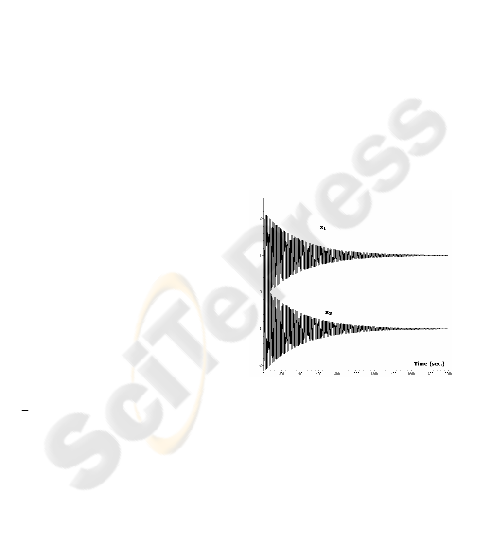
where its optimal solution is
(Xia
Y., 2003). Simulation results are shown in Figures
one and two. For Theorem 2, we used
K=diag{100,100}. From these Figures, we can
appreciate an improvement in the settling time. In all
numerical experiments we employed
)1,1(),(
21
−=
∗∗
xx
,
TT
xxx ]11[)]0()0([)0(
21
==
and
[
][ ]
TT
yyyy 111)0()0()0()0(
321
==
.
3 CONCLUSIONS
We presented a slightly modification to Lagrangian
networks to solve nonlinear convex programming
problem with linear equality constraints. This
modification was able to improve notoriously the
settling time.
Figure 1: Simulation results using Theorem 1
SETTLING-TIME IMPROVEMENT IN GLOBAL CONVERGENCE LAGRANGIAN NETWORKS
317
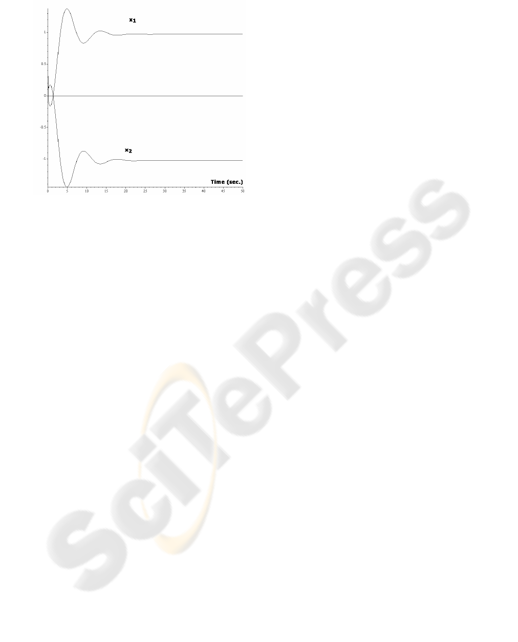
Figure 2: Simulation results using Theorem 2
REFERENCES
M. Krstic, I. Kanellakopoulos, and P. Kokotovic, 1995.
Non-linear and Adaptive Control Design, John Wiley
and Sons. New York.
Y. Xia, 2003. Global Convergence Analysis of Lagrangian
Networks, In IEEE Transaction on Circuits and
Systems I, 50 (6), 818-822, 2003.
ICINCO 2005 - INTELLIGENT CONTROL SYSTEMS AND OPTIMIZATION
318
